Conditional formatting in a Pivot Table is a very useful feature in Microsoft Excel. If you are working on an Excel Report or Excel Dashboard then often require conditional formatting to highlight the values as per our requirements. Today, we will talk about conditional formatting in a Pivot table.
Learn Step by Step Pivot Tables in Excel
Learn Step by Step Conditional formatting in Excel
Conditional Formatting in a Pivot Table
Example 1:
To apply the conditional formatting in a pivot table, just select a cell of value and go to the Home tab >> Conditional formatting>> New Rule
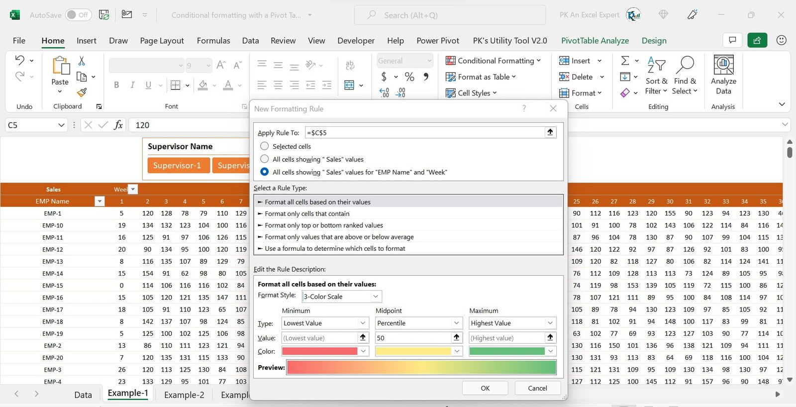
A new formatting Rule window will be opened. There are 3 options for “Apply Rule to”
Selected Cells:
If you select this option then Conditional formatting will be applied only for selected cells. This means it will not be dynamic, it will be always for the selected cells.
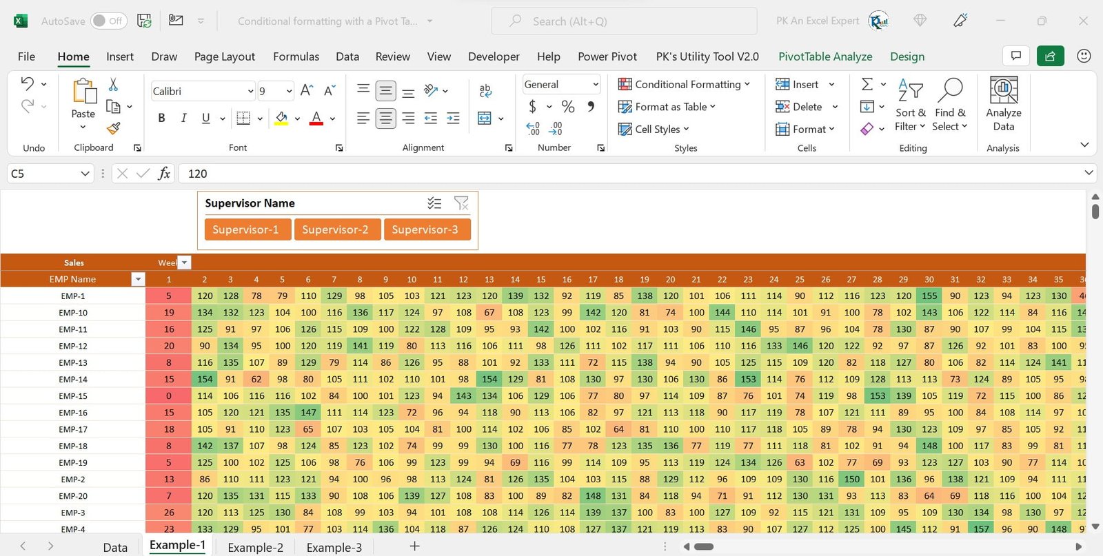
All Cells showing Sales values:
This option can be selected when you want to apply conditional formatting on all the cells wherein the Sales amount is available in an entire pivot table. It will consider the Row and Column Grand Total also for the Sale amount.
All Cells showing Sale values for Emp Name and Week:
You can select this option when you want to apply the conditional formatting only for Emp Name and Week for the Sale amount. t will not consider the Row and Column Grand total also for Sale amount
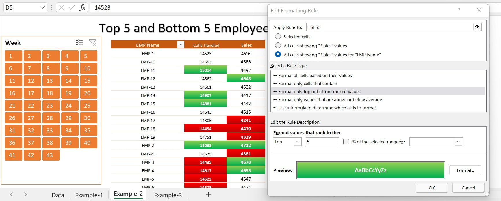
Example 2:
In example 2, we have applied conditional formatting to highlight the Top 5 and Bottom 5 Employee by Call Handled and Sales.
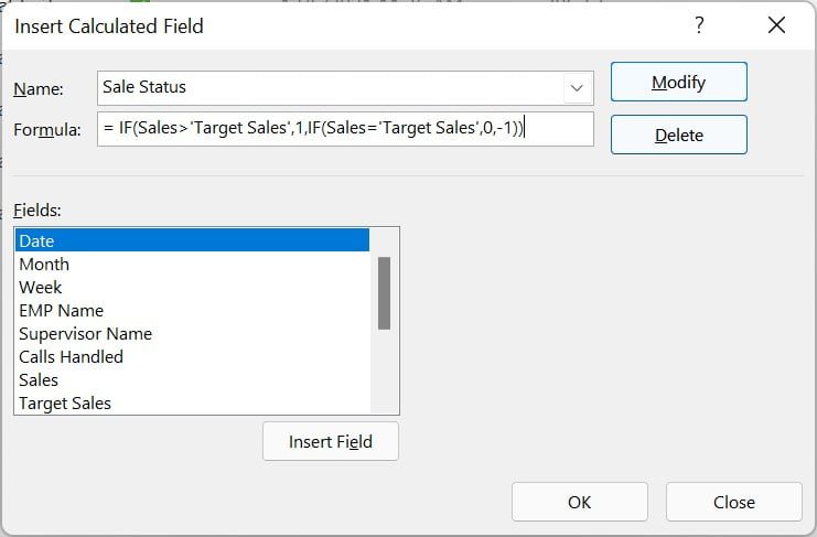
Example 3:
In this example, we have applied 2 types of conditional formatting.
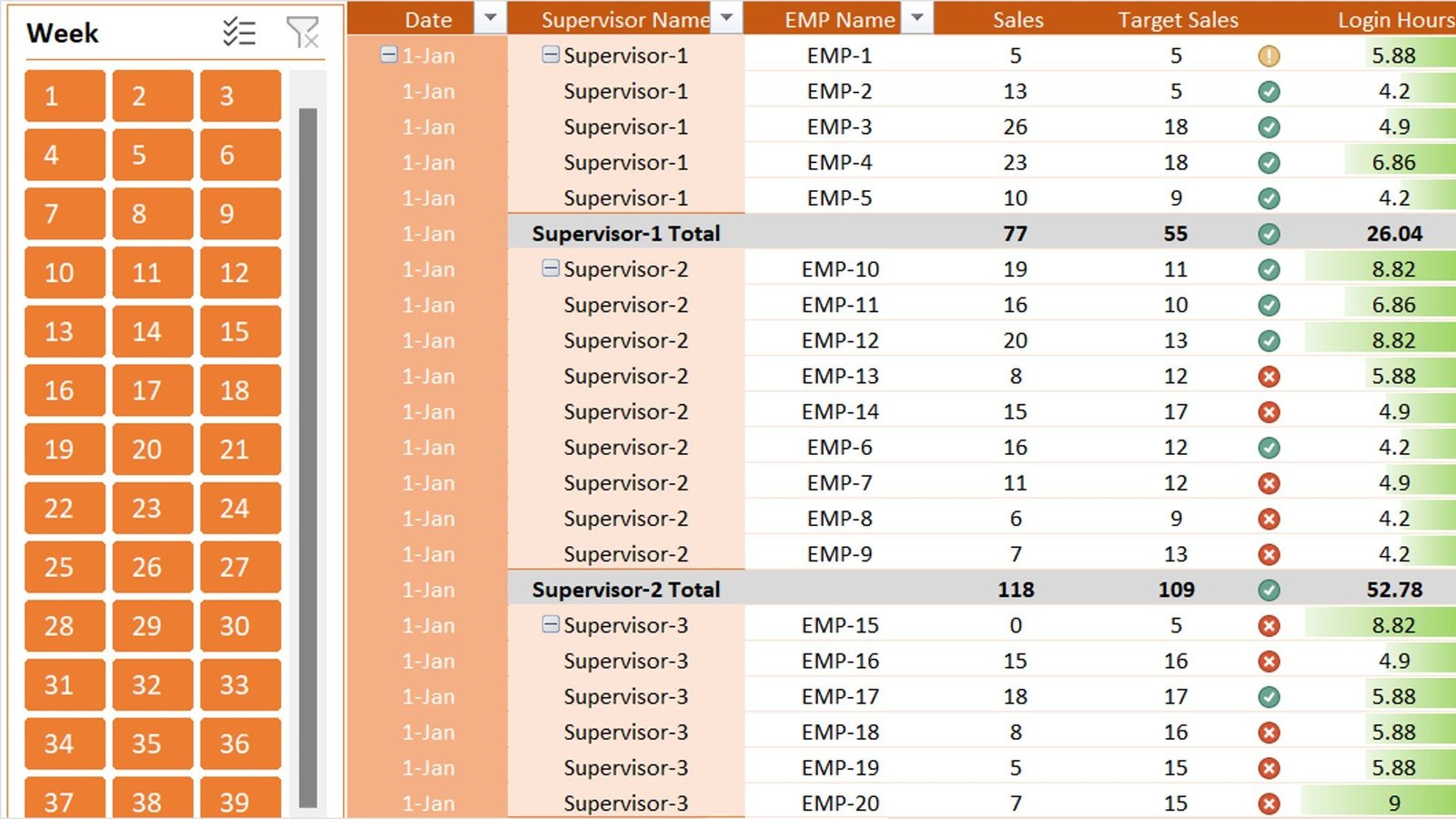
First, we are showing the status for Target Vs Actual Sales with Icon Set in conditional formatting. We have created a Calculated Field first for Sale Status.
To create the Calculated Field, select the pivot table >> go to the Pivot Table Analyze >> Field, Items and Sets >> Calculated Field
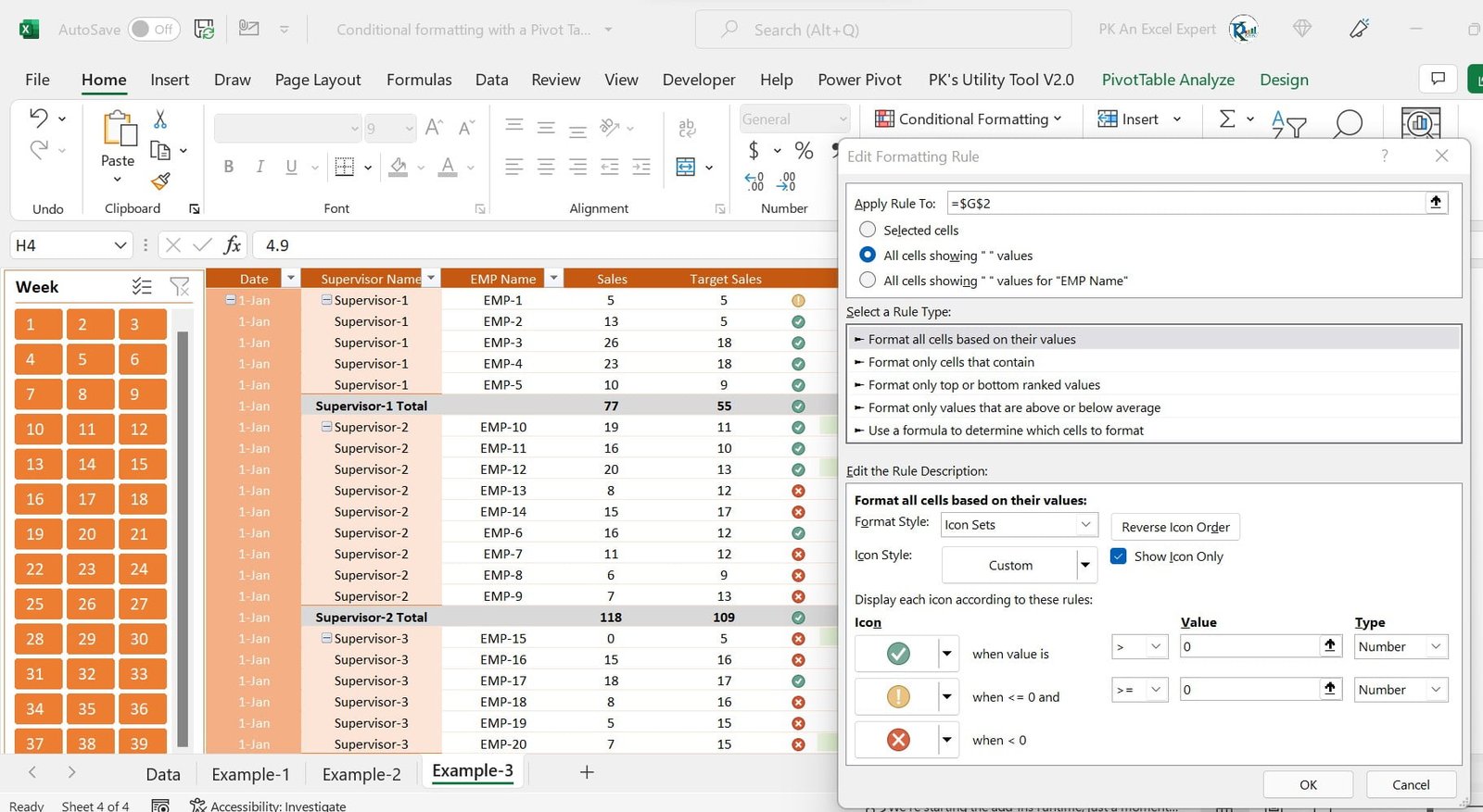
After creating the Calculated field, move this to the pivot table after Target Sales and Rename with space only. Now You can apply a new rule as Icon set as given in the below image-
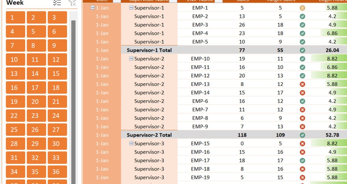
In this example, we have applied Data Bar Conditional formatting also for Login Hours. We are considering the Login hours Target as 9 hours per day.
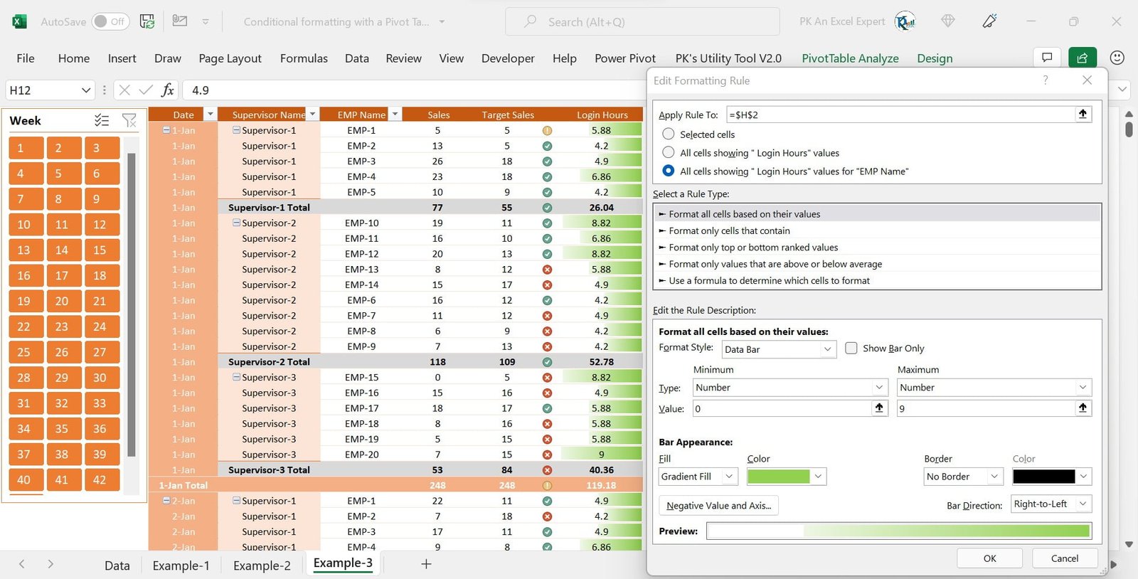
After applying this conditional formatting, our Pivot table will look like this.
Visit our YouTube channel to learn step-by-step video tutorials