“Use a formula to determine which cells to format” rule is used to apply the formatting on the excel cell as our desired condition or a condition which is not available in Excel Conditional Formatting. We have to put a logical formula in the formula box. if this formula returns True then formatting will be applied.
Highlight cells by using formula:
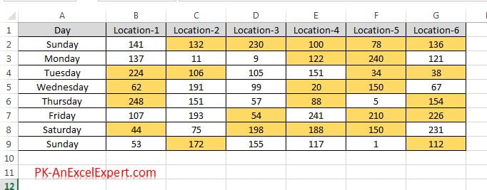
Let’s say we need to highlight the Even number only. Below are the steps-
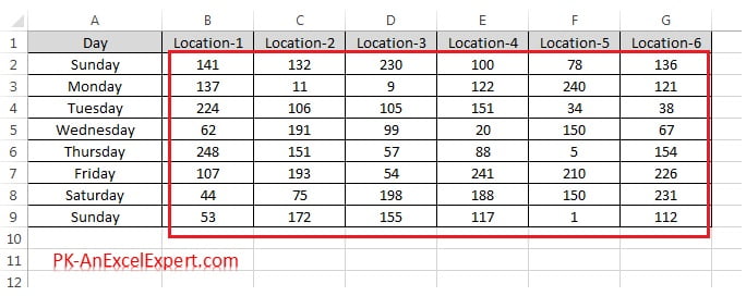
- Select the range on which you want to apply the conditional formatting
- As in below image select “B2:G9”
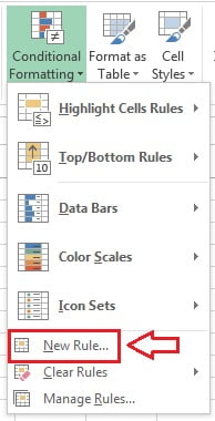
- Go to Home tab>>Conditional Formatting>>New Rules
- New formatting rule window will be opened.
- Select the “Use a formula to determine which cells to format“
- Put formula “=Iseven(b2)” in the box.
- We have taken B2 because it is active cell
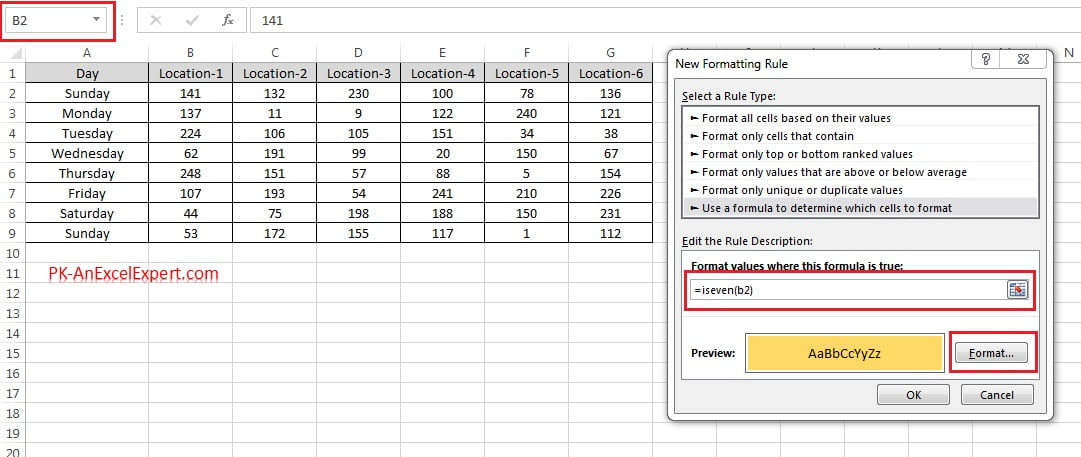
- Click on OK button to apply this conditional formatting.
- Data set with this conditional formatting will look like below image.
Highlight Column by using formula:
we can highlight the column in the selected range by using the formula.
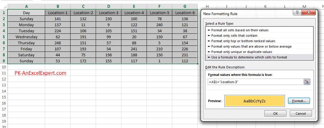
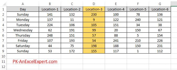
For example, we need to highlight the column which have “Location-3” in the header.
- Select the entire range including headers
- Put the formula =A$1=”Location-3″
- To highlight the column, we have put $ sign before the raw number. That is why we have taken A$1 in the formula.
- Give the format whatever you want to apply in the excel cells.
- Click on OK button to apply this conditional formatting.
- Data set with this conditional formatting will look like below image.
Highlight Row by using formula:
we can highlight the row in the selected range by using the formula.
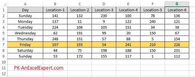
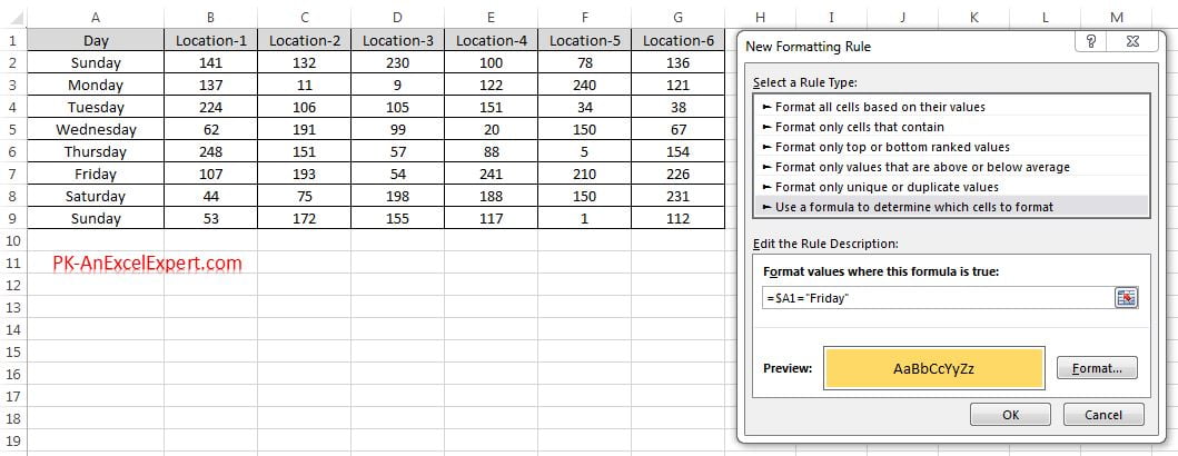
For example, we need to highlight the row for “Friday”
- Select the entire range.
- Put the formula =$A1=”Friday”
- To highlight the row, we have put $ sign before the column (before A). That is why we have taken $A1 in the formula.
- Give the format whatever you want to apply in the excel cells.
- Click on OK button to apply this conditional formatting.
- Data set with this conditional formatting will look like below image.
