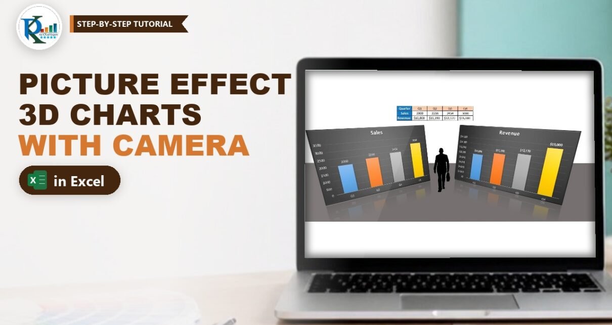
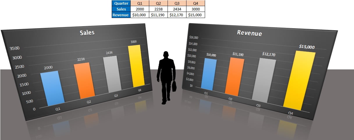
A picture effect in an Excel chart turns a flat column chart into something that looks like a 3D display board standing on a floor, with a reflection underneath. Excel will not let you tilt a normal chart in 3D, but it will let you tilt a picture. The trick is the Camera tool: it takes a live, linked picture of the cells behind your chart, and that picture accepts every picture style, 3-D rotation and reflection Excel has. Because the picture stays linked to the cells, the chart still updates the moment your data changes.
⬇️ Download the Picture Effect Chart File
Two-sheet workbook · .xlsx (no macros) · about 780 KB
Watch the Video Tutorial
In the video PK builds both column charts, adds the Camera to the ribbon, takes linked pictures of the charts, rotates them in 3D, adds the floor and then changes a number to prove the pictures are still live.
What You Will Build
- Two column charts (Sales and Revenue by quarter) with a dark chart style, data labels and a different colour for every column.
- A Camera button on your ribbon, added once and available in every workbook.
- Two linked chart pictures that update automatically when the data changes.
- 3-D rotation and reflection so the charts face each other like display boards.
- A floor and a clean canvas: a dark rectangle sent to the back, with gridlines and headings switched off.
How the Workbook Is Laid Out
The download file has two sheets:
- Picture Effect – the data table and the finished, rotated pictures. The table sits in G1:K3: quarters Q1 to Q4 in H1:K1, Sales (2000, 2238, 2434, 3000) in row 2 and Revenue in row 3.
- Sheet1 – the two real charts. They are only the source; nobody needs to look at this sheet.
Revenue is calculated: H3 holds =H2*5, copied to K3, so Q1 gives $10,000 and Q4 gives $15,000.
Part 1 – Build the Two Column Charts
Step 1: Insert the Sales chart
Select the Quarter row and the Sales row (G1:K2), go to Insert › Charts › Column and pick the first 2-D Clustered Column. You now have one series, Sales, with Q1 to Q4 on the axis.
Step 2: Give it the dark style
With the chart selected, open Chart Tools › Design and choose a dark chart style. PK uses Style 9, the charcoal style with a soft gradient.
Step 3: Add data labels and vary the colours
Right-click the columns and choose Add Data Labels. Then right-click again, choose Format Data Series › Fill & Line and tick Vary colors by point. Each quarter now gets its own colour (blue, orange, grey and gold in the default theme).
Step 4: Build the Revenue chart
Select the Quarter row G1:K1, hold Ctrl and select the Revenue row G3:K3. Insert the same 2-D Clustered Column, apply Style 9, add data labels and tick Vary colors by point.
Step 5: Move the charts to a helper sheet
Select both charts, press Ctrl+X, go to a new sheet and paste. Place each chart so it covers a neat block of cells. In the download file the Sales chart covers Sheet1!C1:J13 and the Revenue chart covers Sheet1!L1:S13. The Camera will photograph these blocks.
Part 2 – Add the Camera Tool to the Ribbon
The Camera command exists in every desktop version of Excel, but it is hidden. You add it once:
Step 6: Open Customize Ribbon
Go to File › Options › Customize Ribbon. In Choose commands from, switch from Popular Commands to Commands Not in the Ribbon.
Step 7: Create a tab and add Camera
Click New Tab on the right side. Excel creates New Tab with a New Group inside it. Find Camera in the left list (the list is alphabetical), select the new group and click Add, then OK. A New Tab now appears on your ribbon with the Camera button in it. You can rename the tab if you like.
Part 3 – Take Linked Pictures of the Charts
Step 8: Photograph the Sales chart
On the helper sheet, select the cells behind the Sales chart (C1:J13 in the file; A1:H15 in the video). Click Camera, go to the Picture Effect sheet and click once where you want the picture. Excel drops a picture of that range, chart included.
Click the picture and look at the formula bar: it shows a reference such as =Sheet5!$A$1:$H$15. That reference is the live link. Whatever happens in those cells, including the chart over them, appears in the picture.
Step 9: Photograph the Revenue chart
Go back, select the cells behind the Revenue chart (L1:S13 in the file; J1:Q15 in the video), click Camera and click on the Picture Effect sheet again.
Step 10: Crop the edges
A camera picture includes every cell in the range, so you may see a strip of empty cells around the chart. Select a picture, click Picture Tools › Format › Crop, drag the black crop handles in to the edge of the chart and click Crop again to finish. Repeat for the second picture.
Part 4 – Add the Picture Effect in Your Excel Chart
This is where the chart becomes a picture effect. Everything below is a normal picture setting, which is why the Camera step matters.
Step 11: Pick a perspective picture style
Select the Sales picture, go to Picture Tools › Format › Picture Styles and open the gallery. Choose a perspective style with a reflection; PK picks the reflected perspective style in the video. The saved file uses a perspective camera, a reflection and a soft top bevel on both pictures.
Step 12: Set the 3-D Rotation for the Sales picture
Right-click the picture, choose Format Picture, open Effects › 3-D Rotation and type:
Sales picture
X Rotation    340°
Y Rotation    10°
Z Rotation    10°
Perspective   100°
Step 13: Set the 3-D Rotation for the Revenue picture
Apply the same picture style to the Revenue picture, then use:
Revenue picture
X Rotation    20°
Y Rotation    10°
Z Rotation    350°
Perspective   100°
How the rotation settings work
- X Rotation turns the picture left or right around a vertical axis. 340° turns the Sales board 20° one way and 20° turns the Revenue board 20° the other way, so the two boards face each other.
- Y Rotation of 10° tips the top of each board slightly away from you.
- Z Rotation spins the picture flat on the screen. 10° and 350° are the same small tilt in opposite directions, which keeps the boards symmetrical.
- Perspective sets the depth: at 100° the near edge looks clearly bigger than the far edge.
Part 5 – Add the Floor and Finish the Scene
Step 14: Draw the floor
Go to Insert › Shapes › Rectangle and drag a wide rectangle from the middle of the charts down to below their reflections. In Shape Fill choose Gray-25%, Background 2, Darker 50% and set Shape Outline to No Outline.
Step 15: Send it to the back
Right-click the rectangle and choose Send to Back. The pictures now stand on the floor and their reflections fall onto it.
Step 16: Clean up the sheet
On the View tab, untick Gridlines and Headings. PK also places a walking businessman silhouette between the boards as a finishing touch.
Step 17: Test the link
Change Q4 Sales from 3000 to another number. The Sales column, the Revenue formula, both charts and both rotated pictures all update together. Your picture effect chart is fully data-driven.
Modern Excel Alternative: Linked Picture
This section is general Excel guidance added to the original tutorial. If you do not want to add the Camera button, you can get the same live picture with Paste Special, as PK mentions in the original post. Select the cells behind the chart, press Ctrl+C, go to the target sheet and choose Home › Paste › Other Paste Options › Linked Picture. The result is identical: a picture with a cell reference in the formula bar that accepts every picture style and 3-D rotation.
Common Errors and Fixes
The picture does not update when the data changes
You probably used Copy as Picture or a normal paste, which creates a static image. Click the picture and check the formula bar. A linked picture shows a reference such as =Sheet1!$C$1:$J$13; if the bar is empty, delete it and use Camera or Linked Picture again.
The picture shows only part of the chart
The chart is bigger than the range you photographed, or it was moved afterwards. Click the picture and edit the reference in the formula bar so it covers the whole chart, then crop again.
3-D Rotation is greyed out
You selected the chart, not the picture. 3-D Rotation is a picture and shape setting. Make sure you click the camera picture on the Picture Effect sheet.
Tips
- Keep the source charts on a separate sheet and hide it when you share the file. The pictures keep working from a hidden sheet.
- Use the same picture style on both boards and mirror the X and Z values (340 and 20, 10 and 350) so the scene looks balanced.
- Microsoft explains the Camera command in Dynamically display the contents of a cell or range in a graphic object.
Want It Ready-Made?
If you need polished charts without building each effect yourself, the Chart Templates in Excel pack on NextGenTemplates.com is a good starting point, and the Charts and Visualization templates collection has more infographic charts. To learn charts, infographics and dashboard design step by step, join the video course Excel Pivot Tables & Dashboards: Basic to Advanced on NextGenTemplates Academy.
Related Tutorials
- Dynamic Graph with Camera in Excel
- Column Chart in Excel
- Advanced Excel Charts and Infographics
- Speedometer Chart in Excel
- Excel Dashboard Design Principles
Frequently Asked Questions
How do I add a picture effect to a chart in Excel?
Take a linked picture of the cells behind the chart with the Camera tool or Paste Special Linked Picture. The picture accepts picture styles, reflection and 3-D Rotation, and it still updates when the chart changes.
Where is the Camera tool in Excel?
It is hidden by default. Go to File, Options, Customize Ribbon, choose Commands Not in the Ribbon, select Camera and add it to a new custom group or to the Quick Access Toolbar.
Will the chart picture update when my data changes?
Yes. A camera picture is linked to a cell range, so any change in the data, the chart or the cells shows up in the picture straight away.
Why can I not apply 3-D Rotation to a normal Excel chart?
3-D Rotation is a picture and shape effect, not a chart setting. Turning the chart into a linked picture is what makes the rotation, perspective and reflection available.
What rotation values make the two charts face each other?
In this tutorial the Sales picture uses X 340, Y 10, Z 10 and the Revenue picture uses X 20, Y 10, Z 350, both with a perspective of 100 degrees.
About the Author
PK is a Microsoft Excel expert and trainer and the founder of PK: An Excel Expert and NextGenTemplates.com. He has been teaching Excel, Power Query and Power BI since 2016 on his YouTube channel.
Conclusion
A picture effect in an Excel chart comes down to one idea: make the chart a linked picture, then style the picture. Build the charts, add the Camera, photograph the chart ranges, apply a perspective style and the 3-D rotation values, and finish with a floor. You get a presentation-ready visual that still updates with your data. Download the file and try your own rotation angles.