Part of the free Module 8: Basic Charts · Lesson 3 of 12 · Full Excel course
Updated on 5 September 2026 · Works in Excel 365, 2021, 2019 and 2016 unless noted.
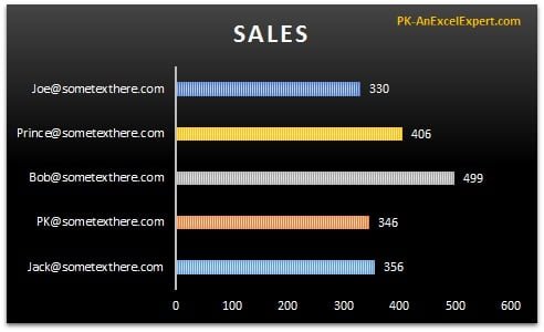
A bar chart in Excel compares values across categories using horizontal bars, with the category names listed down the left and the values running to the right. It is the best basic chart for long labels, rankings and lists of ten or more items. This lesson builds a clustered bar chart of sales by email ID, then formats it: data labels, one colour per bar, reversed category order, gap width and a dark style.
What a bar chart is and when to use it
A bar chart is a column chart turned on its side. Categories run down the vertical axis and values extend horizontally. Because text reads left to right, a label of any length fits beside its bar without wrapping or tilting, which is why bar charts suit email addresses, full names, product descriptions, countries and survey statements. A bar chart also handles more categories than a column chart because the chart can simply grow taller. The steps below are identical in Excel 2016, 2019, 2021 and Microsoft 365; only the tab names differ slightly in older versions.
Sample data for the bar chart
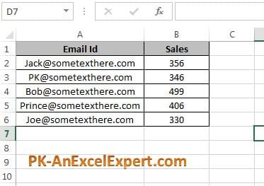
Type this small table into a blank sheet, with the headers in row 1 and the five records in rows 2 to 6. The email IDs are deliberately long so you can see why a bar chart beats a column chart for this kind of label.
| Email ID (A) | Sales (B) |
|---|---|
| [email protected] | 48,500 |
| [email protected] | 62,300 |
| [email protected] | 35,900 |
| [email protected] | 71,200 |
| [email protected] | 54,800 |
Step by step: create a clustered bar chart
- Select the data range including the headers, A1:B6. Including the header row lets Excel name the series and the axis automatically.
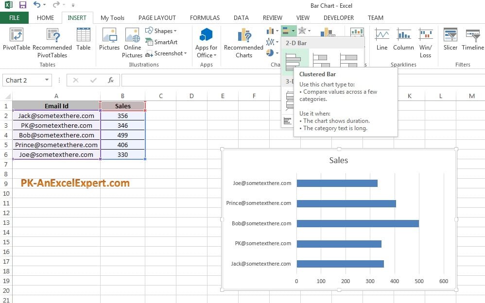
- Go to Insert > Charts > Insert Column or Bar Chart > 2-D Bar > Clustered Bar. Excel drops a chart onto the sheet with one bar per email ID.
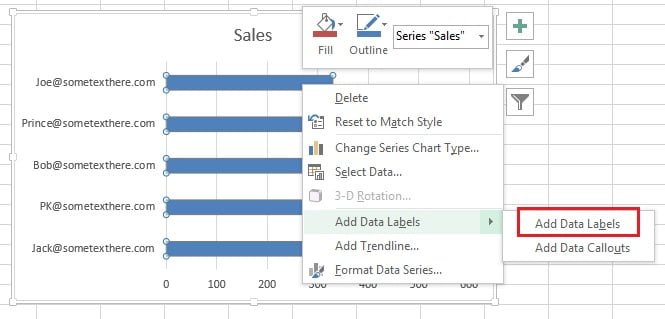
- Right-click any bar and choose Add Data Labels. The sales value appears at the end of each bar, so the reader no longer has to estimate from the axis.
- Right-click a bar again and choose Format Data Series. The Format Data Series pane opens on the right.
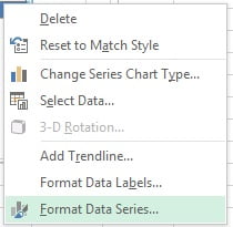
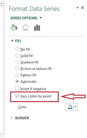
- Under Fill & Line > Fill, tick Vary colors by point so each email ID gets its own colour. Use this only when each bar is a separate entity the reader must track; for a plain ranking a single colour is cleaner.
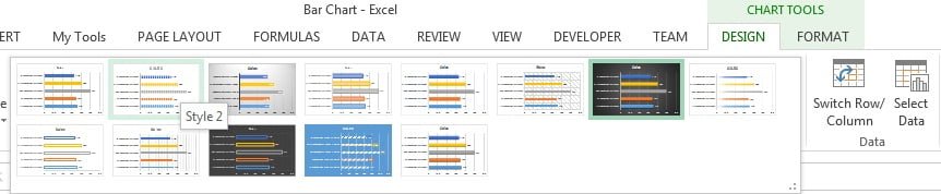
- Click the chart, open the Chart Design tab (called Design under Chart Tools in Excel 2016 and 2019) and pick Style 2 from the Chart Styles gallery.
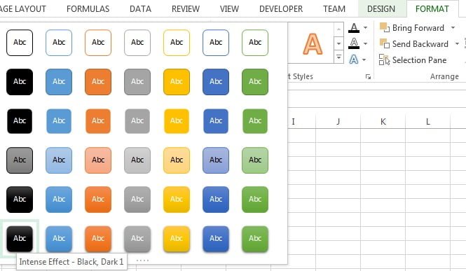
- For a dark background, select the chart, open the Format tab and in Shape Styles choose Intense Effect – Black, Dark 1 (first column, last row). Switch the axis and label fonts to white so they stay readable.
Formatting a bar chart: order, gap width and axis
Three settings turn a default bar chart into a professional one. The most important is category order. Excel plots the first row of your table nearest the origin, which in a bar chart is the bottom, so the chart reads upside down compared with the table.
- Right-click the vertical (category) axis and choose Format Axis.
- Under Axis Options, tick Categories in reverse order. The first email ID now sits at the top. Excel moves the value axis to the top of the plot at the same time; if you prefer it at the bottom, set Horizontal axis crosses to At maximum category.
- Right-click a bar, choose Format Data Series and set Gap Width to between 40% and 60%. The default 150% leaves thin bars with a lot of white space.
- To rank the bars, sort the source data on the Sales column (Data > Sort & Filter > Sort Largest to Smallest). With reverse order ticked, the biggest bar is at the top.
- If data labels are on, click the horizontal (value) axis and press Delete; the labels carry the numbers and the chart looks cleaner. Keep the value axis starting at zero whenever it is visible.
| Setting | Where to find it | Recommended value |
|---|---|---|
| Categories in reverse order | Format Axis > Axis Options (vertical axis) | Ticked, so row 1 appears on top |
| Gap Width | Format Data Series > Series Options | 40% to 60% |
| Data labels | Right-click bar > Add Data Labels, or Chart Elements (+) | Outside End |
| Value axis minimum | Format Axis > Bounds (horizontal axis) | 0 |
| Sort order | Sort the source data, not the chart | Largest to smallest for rankings |
Download the practice file
Download the Bar Chart Excel file to practise with the same data, or click the chart below.
When to use a bar chart and when not to
Choose a bar chart when the category names matter and the reader needs to compare sizes at a glance. Choose something else when the message is a trend or a share of a whole.
| Situation | Bar chart? | Better choice |
|---|---|---|
| Long labels (emails, names, product descriptions) | Yes | Bar chart is the best option |
| Ranking or top-N list | Yes | Sorted bar chart |
| Ten or more categories | Yes | Bar chart, it can grow taller |
| Values over time (months, years) | No | Column chart or line chart |
| Parts of a total | No | Stacked bar chart or pie chart |
| Negative and positive values mixed | Yes, with care | Bar chart with the axis at zero and labels inside the base |
Worked example: top-five sales ranking
A manager wants the five email IDs ranked from highest to lowest sales, with the top performer on the first line. Using the sample data above:
- Click any cell in column B and choose Data > Sort & Filter > Sort Largest to Smallest. The rows are now neha.gupta (71,200), priya.verma (62,300), vikram.patel (54,800), rahul.sharma (48,500), amit.kumar.singh (35,900).
- Select A1:B6 and insert a Clustered Bar chart as in step 2 above.
- Right-click the vertical axis, choose Format Axis and tick Categories in reverse order, so neha.gupta is at the top.
- Add data labels, set Gap Width to 50% and delete the value axis.
- Click the chart title and type Sales by Email ID (Top 5).
Result: five bars in descending order, the longest at the top with 71,200 at its tip, and every email address fully readable on the left. The total range from 35,900 to 71,200 is obvious without reading a single gridline.
Tips and common mistakes
- Include the header row. Excel then uses “Sales” as the series name and picks up the category labels; leave it out and you get “Series1” and numbers 1 to 5.
- Sort the data, not the chart. A bar chart mirrors the sheet order. Sort the table and the chart updates; there is no sort option inside the chart itself.
- Reverse the category order. Almost every bar chart looks wrong until Categories in reverse order is ticked, because Excel starts at the bottom.
- Avoid 3-D bars. The perspective shifts the bar ends away from the gridlines and makes values hard to judge.
- Use one colour for a ranking. Vary colors by point is useful when bars are separate entities; for a top-N list it just adds noise.
- Convert the source to an Excel Table (Ctrl+T). New rows are added to the chart automatically, which is the simplest dynamic range there is.
- Keep the value axis at zero. A truncated axis exaggerates small differences and misleads the reader.
Errors and how to fix them
| Problem | Cause | Fix |
|---|---|---|
| Chart is upside down compared with the table | Excel plots row 1 nearest the origin (bottom) | Format Axis > Categories in reverse order |
| Bars are very thin with wide gaps | Default Gap Width of 150% | Format Data Series > Gap Width 40% to 60% |
| Labels show 1, 2, 3 instead of email IDs | Category column not selected, or header missing | Chart Design > Select Data > Edit the Horizontal (Category) Axis Labels |
| Email IDs are cut off with an ellipsis | Plot area too narrow for the label width | Widen the chart, or drag the plot area boundary to the right |
| Value axis moved to the top | Reverse order also flips the crossing point | Format Axis > Horizontal axis crosses > At maximum category |
| Numbers plotted as a second set of bars | Sales stored as text or two numeric columns selected | Convert text to numbers; select only the columns you need |
Practice exercise
- Retype the sample table and build the clustered bar chart, then add data labels and set Gap Width to 50%.
- Sort the sales largest to smallest and tick Categories in reverse order so the top seller is on the first line.
- Add a third column, Target, with 60,000 in every row, extend the chart to A1:C6 and compare Sales against Target as two bars per email ID.
- Convert the range to an Excel Table with Ctrl+T, add a sixth email ID and confirm the chart grows by itself.
- Apply the dark Shape Style and change the label font to white, then save the chart as a template for reuse.
Key takeaways
- A bar chart is a horizontal column chart; use it for long labels, rankings and long lists.
- The path is Insert > Charts > Insert Column or Bar Chart > 2-D Bar > Clustered Bar.
- Tick Categories in reverse order so the first row of the table appears at the top.
- Set Gap Width to 40% to 60% and add data labels, then remove the value axis for a clean look.
- Sort the source data to rank the bars; the chart follows the sheet order.
- Keep the value axis at zero and avoid 3-D effects.
Related lessons
- Basic Charts course hub
- Column chart in Excel
- Stacked bar chart in Excel
- Chart elements and formatting in Excel
- Dynamic chart range with a Table or named range
- Excel Dashboard course
- SUMIFS function for summarising sales before charting
- Microsoft Support: Create a chart from start to finish
Frequently asked questions
Why is my bar chart in the opposite order to my table?
Excel plots the first category nearest the origin, which is the bottom of a bar chart, so the chart looks flipped. Right-click the vertical axis, choose Format Axis and tick Categories in reverse order. If the value axis jumps to the top, set Horizontal axis crosses to At maximum category to move it back down.
How do I make the bars thicker in an Excel bar chart?
Right-click a bar, choose Format Data Series and reduce the Gap Width. The default is 150%, which gives thin bars; 40% to 60% gives solid bars with a small gap. A Gap Width of 0% makes the bars touch, which suits histograms but not category comparisons.
How do I sort a bar chart from largest to smallest?
Sort the source data, not the chart. Click a value cell and use Data > Sort Largest to Smallest, then tick Categories in reverse order so the largest bar sits at the top. If the data is an Excel Table, the chart re-sorts every time you re-sort the table.
Can I show two measures side by side in a bar chart?
Yes. Select the category column plus two value columns, for example Sales and Target, and insert a Clustered Bar chart. Each category then shows two bars in different colours with a legend. For three or more measures consider a stacked bar chart or a separate chart per measure to avoid clutter.
What is the difference between a bar chart and a column chart in Excel?
They plot the same data; a bar chart uses horizontal bars and a column chart uses vertical ones. Use a column chart for time-based categories such as months, because readers expect time to run left to right. Use a bar chart for long text labels, rankings and lists with many categories.
Want the finished version? Ready-made Excel dashboards, trackers and chart templates are available at NextGenTemplates.com.