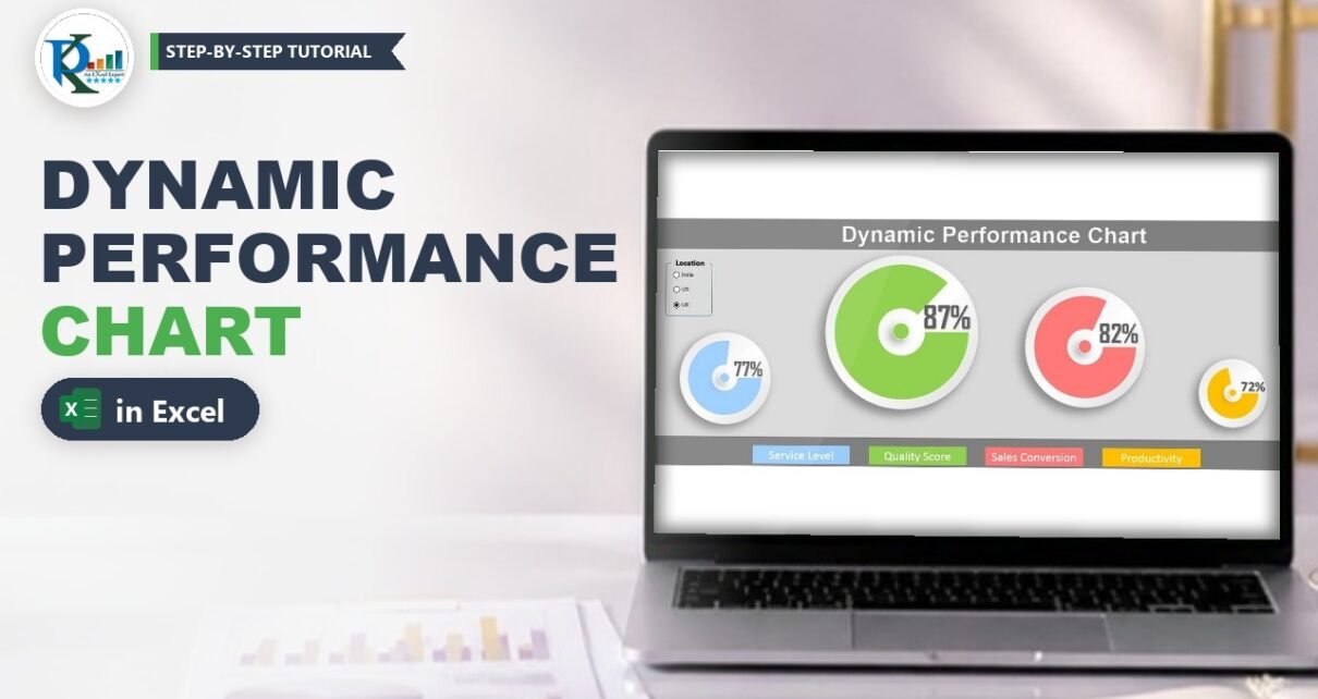
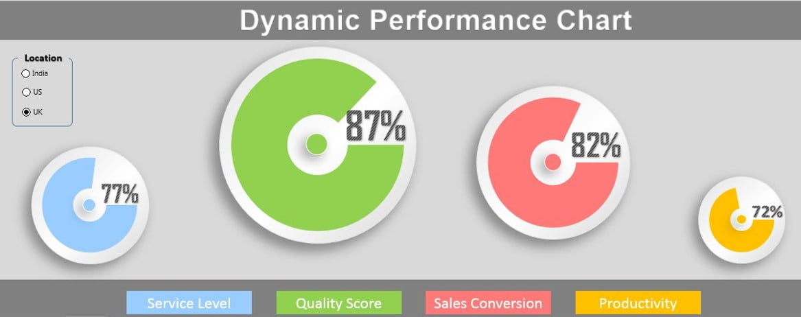
A dynamic performance chart in Excel turns a dull table of KPIs into four stylish circle charts that change the moment you click a different location. In this tutorial you build PK’s version step by step: a small data table, three option buttons for India, US and UK, an INDEX and VLOOKUP helper table, and doughnut charts placed on soft gradient circles with the percentage shown in large WordArt. It needs no VBA and fits straight into a daily report or dashboard.
Watch the Video Tutorial
PK prepares the data with a lookup ID, adds Form Control option buttons, builds the calculation table with INDEX and VLOOKUP, then designs the first circle chart and copies it for the other three metrics.
What You Will Build
- A data table with Location, Metrics and Performance, plus a combined ID column.
- Three option buttons (India, US, UK) linked to one cell.
- A helper table that pulls the selected location’s numbers with INDEX and VLOOKUP.
- Four circle charts made from a doughnut chart, a gradient oval and a coloured centre dot.
- Live percentage labels using WordArt linked to cells.
Part 1: Prepare the Data
Step 1: Enter the performance data
On a sheet (PK uses Sheet3 for all calculations), put the headers Location, Metrics and Performance in row 1. Enter 12 rows, one for each location and metric: India, UK and US, each with Service Level, Quality Score, Sales Conversion and Productivity.
Step 2: Add a unique ID column
Each metric name appears three times, once per location, so you cannot look it up on its own. Insert a column at A (the data moves to B:D), call it ID, and in A2 enter:
=B2&C2Fill it down to A13. The ampersand joins the location and the metric into one unique key, such as IndiaService Level or USProductivity.
Part 2: Design the Report Sheet and Option Buttons
Step 3: Paint the background
Insert a new sheet for the report (Sheet4 in the video). Select the first two or three rows and fill them dark grey, fill the large middle area light grey, and fill a band at the bottom dark grey again. Then go to Insert → WordArt, type Dynamic Performance Chart, make the font white and Arial, and place it in the top band.
Step 4: Insert three option buttons
Go to Developer → Insert → Form Controls → Option Button and click on the sheet. Select it and press Ctrl+D twice to make two copies. Right-click each one, choose Edit Text and rename them India, US and UK.
Draw a rectangle (or a rounded rectangle; drag its yellow handle to change the corner radius) around the buttons with a thin black outline and the background colour or no fill. Select the buttons and use Align Left and Distribute Vertically. Finally add a text box with the caption Location, centred, with the same fill as the background and no outline.
Step 5: Link the buttons to a cell
Right-click any option button, choose Format Control → Control, and set the Cell link to Sheet3!$J$1. Option buttons on the same sheet share one link, so J1 now shows 1 for India, 2 for US and 3 for UK.
Part 3: Build the Helper Table
Step 6: Turn the button number into a location name
Type the list India, US, UK in Q1:Q3, in exactly the same order as the buttons. In K1 enter:
=INDEX(Q1:Q3,J1)How it works: INDEX returns the item at the position given by J1 from the list. Click US and J1 becomes 2, so K1 shows US.
Step 7: Look up the performance with VLOOKUP
Copy the four metric names to J3:J6 with the header Metrics in J2, and add the headers Performance in K2 and Blank Area in L2. In K3 enter:
=VLOOKUP($K$1&J3,$A$1:$D$13,4,0)How the formula works:
$K$1&J3builds the same kind of key as the ID column, for example USService Level. K1 is locked with F4 so it stays fixed when you fill down.$A$1:$D$13is the data table, also locked.4returns the fourth column, Performance.0forces an exact match.
Fill it down to K6 and format as percentages.
Step 8: Calculate the blank area
The doughnut needs two values: the achieved part and the rest. In L3 enter =1-K3 and fill down. With 72% performance the blank area is 28%, and the two always add up to 100%.
Part 4: Create the Dynamic Performance Chart Circles
Step 9: Draw the gradient oval
On the report sheet go to Insert → Shapes → Oval and hold Shift while drawing to get a perfect circle. Set the outline to light grey. Right-click, choose Format Shape → Fill → Gradient fill, pick a preset, and remove stops until only three remain. Move the middle stop to the centre and colour the stops light grey, white and light grey (make the outer stops a touch darker). PK uses a Linear type at a 90° angle.
Then open Effects → Shadow, choose an outer shadow and set the transparency to about 65%, the size to about 103%, the blur to about 15 pt and the distance to 4 or 5 pt.
Step 10: Insert the doughnut chart
On Sheet3 select J3:L3 (Service Level, its performance and its blank area) and insert a Doughnut chart. Remove every chart element (title, legend), set the shape outline to No outline, and give the chart the same height and width, for example 3 by 3, so the doughnut stays round. Right-click the ring, choose Format Data Series, and set the Doughnut Hole Size to 30%.
Step 11: Place the doughnut on the oval
Cut the chart, paste it on the report sheet, and set its chart area to No fill and No outline. Hold Shift to resize it and place it over the oval.
In Format Data Series set the Angle of first slice to 90°. Click the blank-area slice and give it No fill, so only the achieved part shows. Colour the performance slice; PK picks a sky blue from More Fill Colors for Service Level.
Step 12: Add the centre dot and group
Duplicate the oval, shrink it to a small dot, fill it with the same sky blue and place it in the middle of the doughnut hole. Select the chart, the dot and the big oval, then use Format → Align Center and Align Middle, right-click and Group.
Step 13: Add the live percentage
Insert a WordArt, select its border, click in the formula bar, type =, go to Sheet3 and click K3, then press Enter. The WordArt now shows the Service Level percentage and updates with every button click. PK makes it bigger, uses the Agency FB font in bold, reapplies a WordArt style, moves it beside the hole, and groups it with the circle.
Part 5: Copy for the Other Three Metrics
Step 14: Duplicate and resize
Duplicate the finished group three times and resize each copy while holding Shift, so the circles keep their shape. PK uses different sizes for a playful layout.
Step 15: Point each copy to its metric
Right-click a copied chart, choose Select Data → Edit, and change the series. For Quality Score the series name is =Sheet3!$J$4 and the values are =Sheet3!$K$4:$L$4. Link that circle’s WordArt to K4 (PK uses a font size of about 40 on the biggest circle) and recolour the slice and the dot green. Repeat with rows 5 and 6 for Sales Conversion and Productivity in red and amber.
Step 16: Add the legends
In the bottom band add a text box or WordArt for each metric, with white text on a fill that matches its chart colour: Service Level, Quality Score, Sales Conversion and Productivity. Now click India, US and UK to test.
Modern Excel Alternative
This section is an addition from general Excel knowledge; it is not covered in the video.
In Excel 365 or 2021 you can skip the ID column and use XLOOKUP with two conditions, or keep the ID and replace VLOOKUP with =XLOOKUP($K$1&J3,$A$2:$A$13,$D$2:$D$13), which does not depend on a column number. You can also replace the helper list in Q1:Q3 with =CHOOSE(J1,"India","US","UK").
Common Errors and Fixes
Additions from general Excel practice; not shown in the video.
#N/A in the Performance column
The lookup key does not match an ID exactly. Check for extra spaces in the location or metric names, and that the country list spells the names the same way as the data.
The wrong country appears
The order of the list in Q1:Q3 must match the order of the option buttons, because J1 holds only a position number.
The WordArt shows text like =Sheet3!K3
You typed the formula inside the WordArt text. Select the WordArt border first, then type the formula in the formula bar.
Tips
- Keep the chart height and width equal every time you resize, or the ring turns into an oval.
- Hide Sheet3 or move the helper table away from view once the report works.
- Microsoft’s VLOOKUP function reference explains every argument used in Step 7.
Want It Ready-Made?
If you would rather start from the finished file, the Dynamic Performance Chart in Excel on NextGenTemplates.com includes the four circle charts, the option buttons and the formulas from this tutorial. For more infographic and dynamic charts, browse the Excel chart templates. To build complete dashboards with charts like these, PK’s Excel Pivot Tables and Dashboards course takes you from data to finished report.
Related Tutorials
- Doughnut Chart in Excel
- Excel Form Controls: Combo Box, Spin Button and Option Buttons
- Dynamic Chart with a Form Control Scroll Bar
- Stylish Progress Bar Chart in Excel
- Candle Infographic Chart in Excel
Frequently Asked Questions
How do I make a chart change with an option button in Excel?
Link the option buttons to one cell through Format Control, convert that number to a name with INDEX, and use the name in lookup formulas that feed the chart. The chart updates whenever the linked cell changes.
Why do I need an ID column for the lookup?
Each metric name repeats for every location, so VLOOKUP would always return the first match. Joining location and metric creates a unique key for each row.
How do I make a doughnut chart look like a progress circle?
Chart two values, the performance and one minus the performance, set the angle of the first slice to 90 degrees, and give the remaining slice no fill so only the achieved part is visible.
Where do I find the option button in Excel?
On the Developer tab, under Insert and Form Controls. If the Developer tab is hidden, turn it on in File, Options, Customize Ribbon.
Does this dynamic chart need VBA?
No. It uses only Form Controls, INDEX, VLOOKUP, shapes and doughnut charts, so it works in a normal .xlsx file.
About the Author
PK is a Microsoft Excel expert and trainer and the founder of PK: An Excel Expert and NextGenTemplates.com. He has been teaching Excel, VBA, Power Query and Power BI since 2016 on his YouTube channel.
Conclusion
You have built a dynamic performance chart in Excel from scratch: a data table with a lookup ID, option buttons linked to a cell, an INDEX and VLOOKUP helper table, and four doughnut-based circle charts with live WordArt percentages. Swap in your own KPIs and locations, and you have an eye-catching, clickable summary for any report or dashboard.