Dynamic Chart with Scroll Bar in Excel: Form Control Method

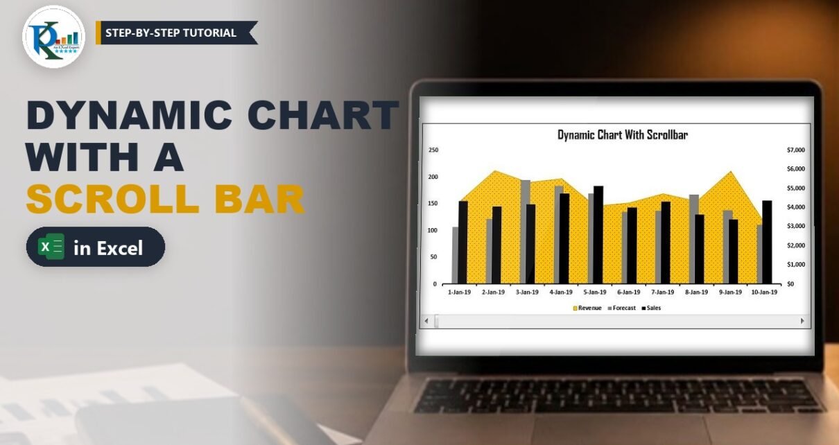
A dynamic chart with scroll bar lets you show a long daily data set in a small, readable chart: drag the scroll bar and the chart slides forward or back one day at a time. In this tutorial you build one in Excel with a Form Control scroll bar, a 10-row helper table driven by INDEX and ROW, and a combo chart that shows Sales and Forecast as columns and Revenue as a patterned area. The data has 120 days, but the chart always shows a clean rolling window of 10 dates. No VBA is needed.

Watch the Video Tutorial

In the video I start from a blank sheet: add the scroll bar, write the INDEX and ROW formula, build the column and area combo chart, then group the scroll bar with the chart and hide the helper columns.

What You Will Build

• A horizontal Form Control scroll bar linked to one cell that holds the starting position.
• A 10-row helper table that pulls the right dates, Sales, Forecast and Revenue from the data sheet with one formula.
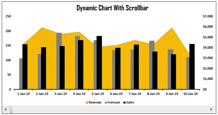
• A combo chart: Sales and Forecast as clustered columns, Revenue as a dotted area on the secondary axis.
• A chart and scroll bar grouped together, so you move and resize them as one object.
• Hidden helper columns while the chart keeps working.

The Sample Data

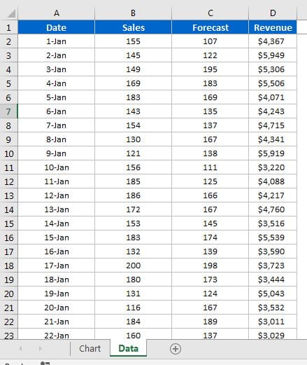
The data sits on a sheet named Data: Date in column A, Sales in B, Forecast in C and Revenue in D, with the headers in row 1. It runs from 1-Jan-2019 to 30-Apr-2019, which is 120 daily rows (A2:A121).

Part 1 – Add the Form Control Scroll Bar

Step 1: Insert the scroll bar

Add a new sheet (the video uses Sheet1) for the chart. Go to Developer → Insert → Form Controls → Scroll Bar and drag a wide, flat rectangle so the scroll bar is horizontal. If you don’t see the Developer tab, turn it on in File → Options → Customize Ribbon.

While you are here, go to View and untick Gridlines so the sheet looks clean.

Step 2: Set the scroll bar options

Right-click the scroll bar, choose Format Control and open the Control tab:

• Minimum value: 1
• Maximum value: based on your data. The video uses 200 for the time being; see the tip below for the exact number.
• Incremental change: 1, so each arrow click moves the chart by one day.
• Cell link: $N$1

Click OK. N1 now shows 1 when the slider is at the far left, and every click on the right arrow adds 1. That single number is the engine of the whole chart.

Tip (my addition): with 120 rows and a 10-day window, the last useful start value is 111, because 111 + 10 points to row 121, the last data row. Set the maximum to 111 and the chart can never scroll past the end into empty rows.

Part 2 – Build the Helper Table for the Dynamic Chart with Scroll Bar

Step 3: Copy the headers

Copy the four headers from the Data sheet and paste them into O1:R1 on Sheet1: Date, Sales, Forecast and Revenue. The chart will read from this small table, not from the full data.

Step 4: Write the first INDEX formula

In O2, a first try looks like this:

O2  =INDEX(Data!A:A,Sheet1!$N$1+1)

INDEX returns the item at a position in a column. With N1 = 1, the position is 2, which is the first date under the header. The +1 skips the header row. Press F4 on the N1 reference so it stays locked when you copy the formula.

The problem appears when you fill it down: every row still uses +1, so all ten rows show the same date. You would have to type +2, +3 and so on by hand.

Step 5: Replace the +1 with ROW

ROW(A1) returns 1. Fill it down and it becomes ROW(A2), ROW(A3) and so on, returning 2, 3 and so on. That is the counter you need. The final formula in O2 is:

O2  =INDEX(Data!A:A,Sheet1!$N$1+ROW(A1))

Copy O2 across to R2, then fill O2:R2 down to row 11 to get 10 rows. Because Data!A:A and A1 are relative, the copies adjust on their own. For example, R2 becomes:

R2  =INDEX(Data!D:D,Sheet1!$N$1+ROW(D1))

The reference inside ROW can be any cell in row 1 (A1, B1, C1). Only the row number matters.

How the formula works

• Sheet1!$N$1 is the scroll bar value, the start position. It is locked with $ so every cell reads the same value.
• ROW(A1) gives 1 in the first row of the table, 2 in the second, up to 10 in the tenth.
• Added together they give the rows to fetch. With N1 = 1 the table shows data rows 2 to 11 (1-Jan to 10-Jan). Click the scroll bar once and N1 = 2, so the table shows rows 3 to 12 (2-Jan to 11-Jan).
• INDEX(Data!A:A, ...) returns the value at that row: the date in column A, Sales in B, Forecast in C and Revenue in D.

Use the Format Painter to copy the formatting from the Data table onto O1:R11, so the dates show as 1-Jan and Revenue as currency. Want 15 days or a full month instead of 10? Fill the formulas down further. Then lower the scroll bar maximum to match.

Part 3 – Create the Combo Chart

Step 6: Insert a clustered column chart

Select O1:R11 and go to Insert → Charts → 2-D Clustered Column. You get three column series: Sales, Forecast and Revenue.

Step 7: Turn Revenue into an area on the secondary axis

Revenue is in dollars and is much bigger than Sales and Forecast, so it needs its own axis. Right-click any column, choose Change Series Chart Type and for Revenue select Area and tick Secondary Axis. Click OK. The units now sit on the left axis and the dollars on the right axis.

Step 8: Format the series

• Delete the chart gridlines.
• Revenue area: right-click, Format Data Series → Fill → Pattern fill. Pick the first dotted pattern, set the foreground to black and the background to Gold (Accent 4). Any colour you like works.
• Sales and Forecast columns: set Series Overlap to about 40% and Gap Width to about 150%.
• Give Forecast a solid grey fill and Sales a solid black fill.

Part 4 – Put the Scroll Bar on the Chart

Step 9: Make room and group

1. Select the plot area and drag its bottom edge up to free some space at the bottom of the chart. Move the legend if it is in the way.
2. Drag the scroll bar onto the chart. If it goes behind the chart, right-click the chart and choose Send to Back. The scroll bar is then on top.
3. Resize the scroll bar to the width of the plot area.
4. Select the chart and the scroll bar together (hold Ctrl), right-click and choose Group.

Finish with a black chart outline, bold black axes and legend, and your own chart title. In my file the title is Dynamic Chart With Scrollbar.

Part 5 – Hide the Helper Columns

Select columns O to R and press Ctrl+0 to hide them. The chart goes blank, because Excel doesn’t plot hidden cells by default. To fix it, right-click the chart → Select Data → Hidden and Empty Cells, tick Show data in hidden rows and columns and click OK twice. The chart is back and the helper table stays out of sight.

Modern Excel Alternative (Microsoft 365)

This section is my addition and is not shown in the video. In Excel for Microsoft 365, one formula in O2 can return the whole 10 x 4 window:

O2  =TAKE(DROP(Data!A2:D121,$N$1-1),10)

DROP removes the first N1 – 1 rows of the data and TAKE keeps the next 10. The result spills into O2:R11, the same range the chart already uses, so the chart works unchanged. Keep O3:R11 empty or you will get a #SPILL! error.

Common Errors and Fixes

All rows show the same date

You used a fixed +1. Replace it with ROW(A1) as in Step 5 so each row adds a different number.

The chart shows 0 or 0-Jan-1900 at the end

The scroll bar maximum is larger than your data. INDEX is reading empty rows. Set the maximum to the number of data rows minus the window size plus 1 (120 – 10 + 1 = 111).

The chart is empty after hiding columns

Turn on Show data in hidden rows and columns under Select Data → Hidden and Empty Cells (Part 5).

Tips

• Set Page change in Format Control to 10 so clicking the empty track jumps a whole window.
• Put the dynamic date range in the chart title, for example with a cell that joins the first and last date of the helper table, so readers always know which days they see.
• The same INDEX + ROW pattern works with a spin button or a vertical scroll bar.
• Microsoft’s page on the INDEX function explains every argument in detail.

Want It Ready-Made?

If you’d rather start from the finished workbook, the Dynamic Chart with Form Control Scrollbar template on NextGenTemplates.com has the data, helper table and grouped chart ready to adapt. You’ll find more interactive charts in the Excel Charts and Visualization collection. To build charts, form controls and full dashboards step by step, join the video course Excel Pivot Tables and Dashboards.

Related Tutorials

• Dynamic Step Chart in Excel: Rolling 7-Day Window
• Fully Dynamic Chart with Scroll Bar and Spin Button
• Show Data Dynamically Using a Vertical Scroll Bar
• Dynamic Chart Range in Excel: Charts That Update Automatically
• Excel Form Controls: Combo Box, Spin Button and Option Buttons

Frequently Asked Questions

How do I add a scroll bar to a chart in Excel?

Insert a Form Control scroll bar from the Developer tab and link it to a cell. Build a small helper table whose formulas read that cell, chart the helper table, then place the scroll bar on the chart, send the chart to back and group both objects.

What should the maximum value of the scroll bar be?

Use the number of data rows minus the number of rows shown plus 1. For 120 days and a 10-day window that is 111, so the last window ends exactly on the last date.

Why use ROW in the INDEX formula?

ROW(A1) returns 1 and grows to 2, 3 and so on as you fill down. Adding it to the scroll bar value gives each row of the helper table its own position in the data.

Can I show more than 10 days?

Yes. Fill the helper formulas down for as many rows as you want, extend the chart range to match and lower the scroll bar maximum by the same amount.

Does this dynamic chart need VBA?

No. It uses a Form Control scroll bar, INDEX and ROW formulas and normal chart formatting. The workbook can be saved as a regular .xlsx file.

About the Author

PK is a Microsoft Excel expert and trainer and the founder of PK: An Excel Expert and NextGenTemplates.com. He has been teaching Excel, Power Query and Power BI since 2016 on his YouTube channel.

Conclusion

A dynamic chart with scroll bar takes only a few pieces: a Form Control scroll bar linked to N1, one INDEX + ROW formula copied into a 10-row helper table, and a column and area combo chart grouped with the scroll bar. Hide the helper columns, tick Show data in hidden rows and columns, and you have a compact chart that can browse months of daily data with one click.