In this article you will learn how to create a dynamic Step Chart in Excel. In this chart we can show the rolling 7 days price or sales.
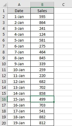
Let’s say we have dates on column A (“1-Jan to 3-Feb”) and sales on column B. For this data set we will create the dynamic step chart.
Below are the steps to create the Dynamic Step Chart in Excel-
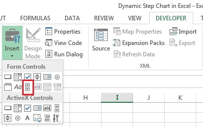
- Go to the Developer Tab>>Insert>>Scroll bar (Form Control)
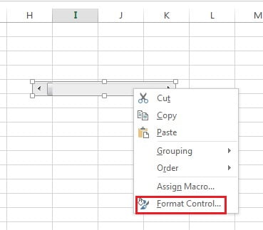
- Drag the scroll bar on the worksheet.
- Right click on the scroll bar and click on Format Control.
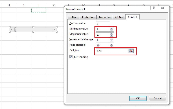
In the Format Control window-
- Put Minimum value as 1.
- Put Maximum value as 27. We are taking 27 here because we have 34 dates in our data set and we will display 7 days on the charts at a time. So “34 – 7 = 27“.
- Cell link as “$J$1”
Now we will create support columns as Date, Sales and Data label to create this chart.
- Create Date on column G.
- Formula for G2 is “=INDEX(A:A,$J$1+1)“
- Formula for G3:G4 is “=INDEX(A:A,$J$1+2)“
- Formula for G5:G6 is “=INDEX(A:A,$J$1+3)“
- Formula for G7:G8 is “=INDEX(A:A,$J$1+4)“
- Formula for G9:G10 is “=INDEX(A:A,$J$1+5)“
- Formula for G11:G12 is “=INDEX(A:A,$J$1+6)“
- Formula for G13:G14 is “=INDEX(A:A,$J$1+7)“
- Create Sales column on H.
- Put formula “=IF(ISEVEN(ROW()),VLOOKUP(G2,A:B,2,0),H1)” on H2.
- Fill down the formula for “H2:H14“
- Create Data Labels column on I.
- Put formula ” =IF(ISEVEN(ROW()),VLOOKUP(G2,A:B,2,0),””) ” on I2.
- Fill down the formula for “I2:I14“

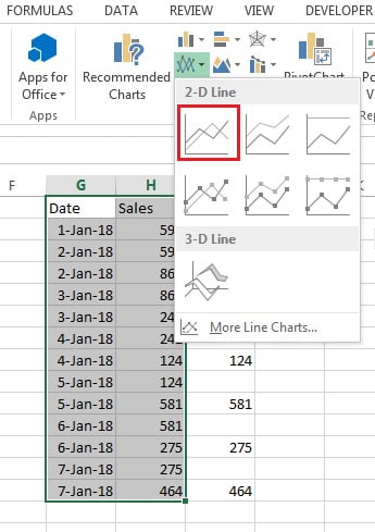
- Select the range “G1:H14”
- Go to the Insert tab>>Charts>>Insert Line Chart(without marker)
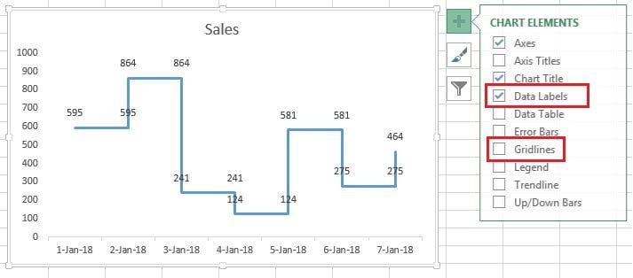
- After inserting the chart successfully, remove the Gridlines and add Data Labels by using Chart Elements (+button) of chart.
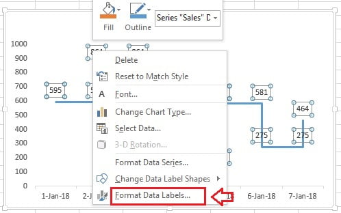
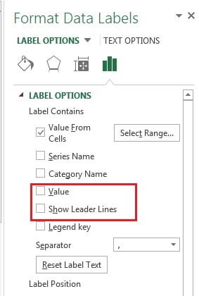
- Right click on the data label and click on Format Data Labels.
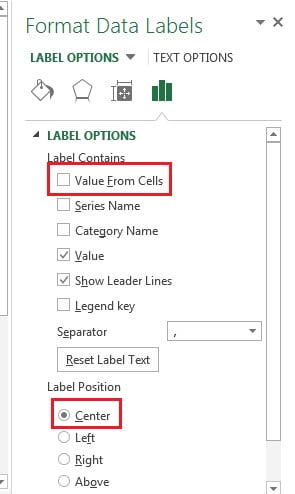
- In Format Data Labels window choose Label Position as Center.
- Tick the Value From Cells available under Label Contains.
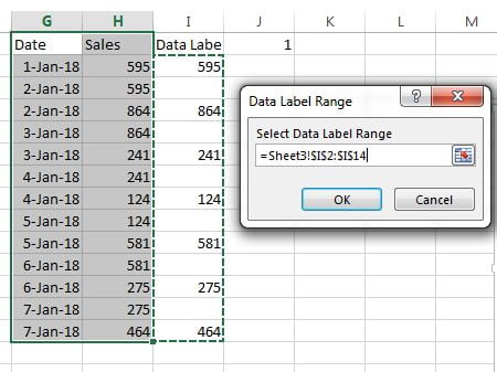
- Data Label Range window will be opened
- Select range I2:I14.
- Now remove the tick from Value and Show Leader Lines available in Format Data Labels window.
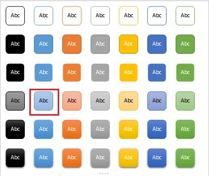
- Now fill the background color in data labels.
- Select the data labels and go to Format Tab>>Shape style>>Choose a light blue color style.
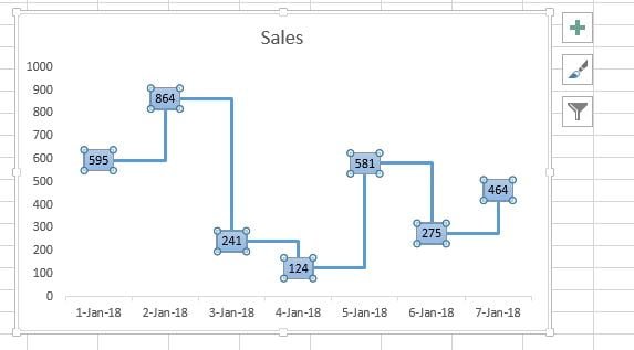
- Chart After formatting the data label will look like blow image.
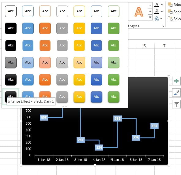
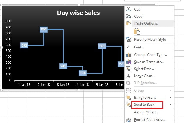
- Now select the entire chart and go to Format Tab>>Shape style>>Choose a Black color style.
- Right click on the chart area and click on Send to back so that Scroll bar will be above the chart.
Click to buy Dynamic Step Chart in Excel
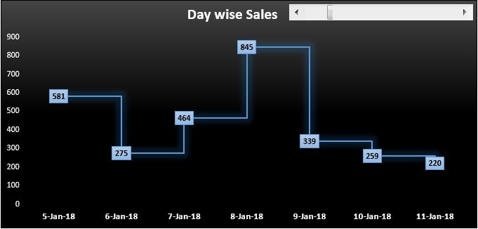
- Put the scroll bar on the Top-Right side.
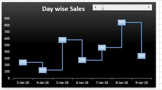
- Select the data label and change the font color as Black.
Our Chart is ready will look like below image-
Click to buy Dynamic Step Chart in Excel
Visit our YouTube channel to learn step-by-step video tutorials
Watch the video tutorial:
Click to buy Dynamic Step Chart in Excel