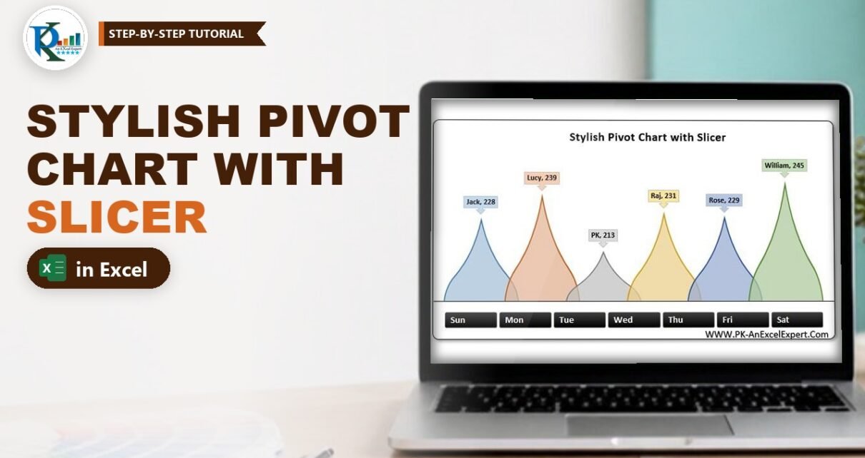
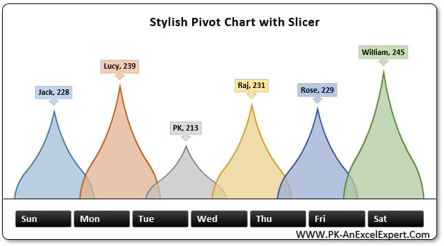
A stylish pivot chart with slicer in Excel turns a plain employee sales report into an eye-catching, clickable visual. In this tutorial you build PK’s teardrop chart step by step: a pivot table of employee-wise sales, a column pivot chart where every employee is a separate series, curved teardrop pictures in place of the bars, callout labels with names and values, and a black-button Day slicer that filters the chart with one click. No formulas and no VBA, just pivot and chart formatting.
Watch the Video Tutorial
In the video PK builds the chart from the raw data: pivot table, pivot chart, teardrop pictures, callout labels, a custom slicer style and a framed, grouped layout.
What You Will Build
- A pivot table that totals sales by employee, in tabular form with no grand totals.
- A pivot column chart with one series per employee, so each column can look different.
- Teardrop columns made from a rotated, cropped shape pasted as a picture.
- Callout data labels that show the employee name and the sales value.
- A seven-button Day slicer with a custom black style, framed together with the chart.
The Data Behind the Chart
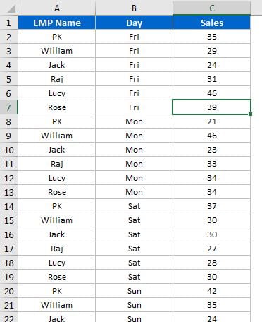
The data sheet is a simple three-column list: EMP Name, Day and Sales. There is one row for each employee and day, for six employees (Jack, Lucy, PK, Raj, Rose and William) across the seven days of the week.
Part 1: Build the Pivot Table and Pivot Chart
Step 1: Insert the pivot table
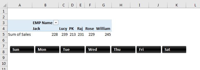
Click inside the data, go to Insert > PivotTable and click OK to place it on a new sheet. Drag EMP Name to Rows and Sales to Values. You now have employee-wise sales: Jack 228, Lucy 239, PK 213, Raj 231, Rose 229 and William 245.
Step 2: Tidy the pivot table
On the Design tab choose Grand Totals > Off for Rows and Columns and Report Layout > Show in Tabular Form. Turn off View > Gridlines for a clean sheet. Removing the grand total matters, because otherwise it would turn into one more column in the chart.
Step 3: Insert a clustered column pivot chart
Select a cell in the pivot table and choose Insert > Column Chart > 2-D Clustered Column. Because the source is a pivot table, Excel creates a pivot chart.
Step 4: Hide the buttons and clean the chart
With the chart selected, go to PivotChart Analyze > Field Buttons > Hide All (the tab was called simply Analyze in Excel 2013). Then click the + Chart Elements button and untick Axes, Gridlines and Legend.
Step 5: Switch rows and columns
Right-click the chart, choose Select Data and click Switch Row/Column, then OK. EMP Name moves to the Legend (Series) area, so each employee becomes a separate series in one category.
Why this step matters: a picture fill and a data label are set per series. With one series per employee you can give every column its own teardrop colour, and the label can show the series name, which is now the employee’s name.
Part 2: Turn the Columns into Teardrops
Step 6: Draw and shape the teardrop
Go to Insert > Shapes > Basic Shapes > Teardrop and draw it. Right-click it, choose Format Shape > Size & Properties and set Rotation to -45° so the point faces straight up. Drag the yellow adjustment handle upward to stretch the point into a tall spike. Then, in the Fill settings, set Transparency to 25%.
Step 7: Paste it as a picture and crop it
Copy the shape (Ctrl + C) and use Home > Paste > Picture, or Paste Special > Picture (PNG). Delete the original shape. Select the picture, click Picture Format > Crop and drag the bottom handle up to about half its height, so you keep the point and the widest part. Click Crop again to finish. The flat bottom will sit on the base of the chart.
Step 8: Paste the picture into each series
Copy the cropped picture, click once on the first column to select that series and press Ctrl + V. The column now shows the teardrop. Select the picture again, open Picture Format > Color and pick a different recolour option, then copy it and paste it into the second column. Repeat until all six columns have their own colour.
Step 9: Overlap the teardrops
Right-click any column and choose Format Data Series. Set Gap Width to 0% and Series Overlap to about 15% (PK suggests 15 to 20). The wide bases now touch and overlap slightly, and the 25% transparency lets you see each shape through its neighbour.
Part 3: Add Callout Labels
Step 10: Add the data labels and change their shape
Right-click the first series and choose Add Data Labels, then repeat for each series. Right-click a label, choose Change Data Label Shape and pick a callout shape with a pointer, so each label points down to its teardrop. Give each label a fill that matches its teardrop, with bold black text.
Step 11: Show the employee name
Right-click a label and choose Format Data Labels. Under Label Options tick Series Name as well as Value. Because each series is an employee, the label reads Jack, 228. Do the same for the other five labels.
Step 12: Remove the chart’s own background
Select the chart and, on the Format tab, set Shape Fill to No Fill and Shape Outline to No Outline. The frame you add in Part 5 will provide the background.
Part 4: Add and Style the Day Slicer
Step 13: Insert the slicer
Select the chart and choose PivotChart Analyze > Insert Slicer, tick Day and click OK. Click any day and the chart shows only that day’s sales.
Step 14: Create a custom slicer style
On the Slicer tab, open the Slicer Styles gallery and choose New Slicer Style. Format two elements:
- Selected Item with Data: a black gradient fill and bold white font.
- Unselected Item with Data: a grey fill and white font.
Click OK, then apply the new style from the gallery. For a full walkthrough, see PK’s guide to creating a custom slicer style in Excel.
Step 15: Turn the slicer into a row of buttons
Right-click the slicer, choose Slicer Settings and untick Display header. On the Slicer tab set Buttons > Columns to 7, one per day. Reduce the height, widen it and place it under the chart.
Part 5: Frame and Group the Stylish Pivot Chart with Slicer
Step 16: Add the frame
Draw a black Line shape along the base of the teardrops. Then insert a Rounded Rectangle around the chart and slicer, drag its yellow handle to make the corners less round, set a white fill and a black outline, and choose Send to Back. Add Shape Effects > Shadow for depth.
Step 17: Group everything
Select the shapes, chart and slicer together (Ctrl + click), then right-click and choose Group, so the whole visual moves as one object. You can now hide the pivot table sheet. To filter several days, Ctrl + click them in the slicer. To show all days again, PK Ctrl + clicks the selected day.
Common Errors & Fixes
- The pasted picture fills every column. You clicked twice and selected all series in one category, or skipped Switch Row/Column. Switch rows and columns, then click a single column once before pasting.
- The label shows Total instead of the name. Category Name is ticked rather than Series Name. Tick Series Name.
- The slicer does not filter the chart. It was inserted from a different pivot table. Right-click the slicer, choose Report Connections and tick the chart’s pivot table.
- An extra Grand Total column appears. Turn Grand Totals off on the Design tab (Step 2).
Tips
- Use 5 to 8 employees. More series make the teardrops too thin to read.
- Keep the transparency between 20% and 30% so overlapping shapes stay readable.
- Save your slicer style once and reuse it on every dashboard in the workbook.
- Microsoft explains the basics of using slicers to filter data.
Want It Ready-Made?
Want the finished workbook with the chart, slicer style and data already built? Get the Stylish Pivot Chart with Slicer in Excel template on NextGenTemplates.com, or browse more Excel charts and visualization templates. To master pivot tables, slicers and dashboard charts step by step, join the course Excel Pivot Tables and Dashboards.
Related Tutorials
- Pivot chart in Excel: create it and hide the field buttons
- 3D container pivot chart with slicer and timeline
- Dynamic sales funnel chart with slicers
- Stylish butterfly chart in Excel (version 1)
- 10 useful pivot table tips
FAQ
How do I make each column in a pivot chart a different shape or colour?
Use Select Data and Switch Row/Column so each item becomes its own series. Then select one series at a time and paste a picture or set its own fill.
Why does the pasted teardrop look stretched?
Excel stretches a pasted picture to the column size. Crop the picture to the part you want to show and keep Gap Width at 0 so the columns are wide enough.
How do I show the employee name on the data label?
Open Format Data Labels and tick Series Name. This works because each employee is a separate series after switching rows and columns.
Can I select more than one day in the slicer?
Yes. Hold Ctrl and click each day you want. In newer Excel versions you can also turn on the Multi-Select button in the slicer header if the header is visible.
Does this chart need VBA?
No. It uses only a pivot table, a pivot chart, shapes, pictures and a slicer, so the file stays a normal macro-free workbook.
About the Author
PK is a Microsoft Excel expert and trainer and the founder of PK: An Excel Expert and NextGenTemplates.com. He has been teaching Excel, Power Query and Power BI since 2016 on his YouTube channel.
Conclusion
A stylish pivot chart with slicer in Excel comes down to one key move, Switch Row/Column, which turns every employee into a separate series. After that you paste a cropped teardrop picture into each series, overlap them, add name-and-value callouts and connect a seven-button Day slicer. Build it once and you have a reusable, click-to-filter visual for any dashboard or presentation.