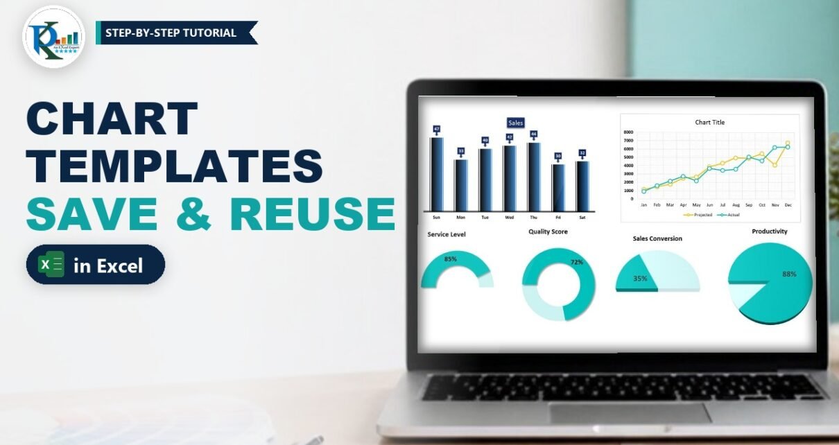
Chart templates in Excel let you format a chart once and reuse that exact look on any new data in a couple of clicks. Instead of removing gridlines, picking colours and styling data labels every time, you save your favourite chart as a template (a .crtx file) and insert it like any built-in chart type. In this tutorial you will save a gradient column chart and a styled line chart as templates, see how ready-made KPI templates work, and learn how to apply, manage and share them as a company standard.
Watch the Video Tutorial
In the video, PK first creates six charts instantly from saved templates, then builds a column chart and a line chart from scratch and saves each one as a new template.
What You Will Build
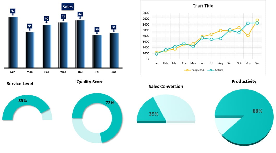
- A gradient column chart template with callout-style data labels, no gridlines and no vertical axis.
- A line chart template with full gridlines, teal and yellow lines and white circle markers.
- KPI chart templates (half doughnut, doughnut and pie) that turn a single percentage into a visual.
- The habit of inserting any saved design from Insert > Recommended Charts > All Charts > Templates.
Why Use Chart Templates in Excel?
Excel’s built-in chart styles are a starting point, but most people end up making the same changes again and again: delete gridlines, thicken lines, change marker shapes, recolour data labels. A chart template stores all of that formatting. Once saved, it is available in every workbook you open on that PC, not just the file where you created it. That makes templates ideal for:
- Recreating your favourite chart design on new data in seconds.
- Creating a company standard chart style so every report looks consistent.
- Styles that are not available in the built-in Chart Styles gallery, such as the custom line and marker design shown below.
How the Sample Workbook Is Organised
The workbook in the video has four sheets: Column Chart, Line Chart, KPI Chart and Example. The first three show finished charts created from templates; the Example sheet is where the two new templates are built.
- Column Chart: Day and Sales for Sun to Sat (47, 33, 40, 42, 44, 30, 32).
- Line Chart: month-wise Projected and Actual sales for Jan to Dec.
- KPI Chart: Service Level 85%, Quality Score 72%, Sales Conversion 35% and Productivity 88%, each with helper cells next to it.
- Example: employee-wise Productivity for EMP-1 to EMP-10, and an Interval table with Forecast and Call Received.
Part 1 – Build and Save a Column Chart Template
Step 1: Insert a clustered column chart
On the Example sheet, select the employee productivity range (EMP and Productivity columns) and go to Insert > Column Chart > 2-D Clustered Column. You get a plain blue column chart with gridlines and a vertical axis.
Step 2: Clean up the chart
- Delete the horizontal gridlines and the vertical axis. The data labels you add later make the axis unnecessary.
- Make the chart title bold, and make the horizontal axis labels bold and black.
Step 3: Narrow the gap and add a gradient fill
Right-click a column and choose Format Data Series. In Series Options set the Gap Width to around 50 or 60 so the columns become wider. Then open Fill & Line > Fill > Gradient fill, keep the type as Linear and build the stops from a near-black colour to blue. This dark-to-blue gradient gives each column a rounded, 3D look.
Step 4: Add and style the data labels
- Add data labels from the chart’s + button.
- Right-click a label and choose Change Data Label Shape, then pick a callout shape so each label points down to its column.
- In Format Data Labels > Fill choose Solid fill with a dark blue colour.
- On the Home tab, set the label font to white and bold.
Step 5: Save as Template
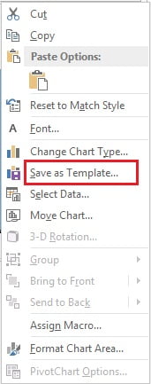
Right-click the chart area and click Save as Template. Excel opens the Charts templates folder. Give the file a clear name (in the video it is called Chart1) and click Save.
Step 6: Test the template
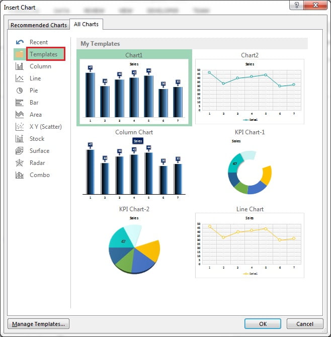
Delete the chart, select the data again and go to Insert > Recommended Charts > All Charts > Templates. Your new template appears under My Templates. Select it and click OK, and the fully formatted chart is back instantly.
Part 2 – Build and Save a Line Chart Template
Step 7: Insert a line with markers
Select the Interval, Forecast and Call Received table and go to Insert > Line Chart > Line with Markers.
Step 8: Turn on the full grid
Click the chart’s + button, open the arrow next to Gridlines and tick all four options: Primary Major Horizontal, Primary Major Vertical, Primary Minor Horizontal and Primary Minor Vertical. The chart now sits on a fine graph-paper grid.
Make the legend, both axes and the chart title bold and black.
Step 9: Format the first line
- Right-click the first line and choose Format Data Series > Fill & Line.
- Under Line choose Solid line and pick a teal colour from More Colors.
- Under Marker > Marker Options choose Built-in, a circle, size 8.
- Set the marker Fill to Solid fill, white.
- Set the marker Border to Solid line in the same teal as the line, width 2.25 pt.
Step 10: Format the second line
Repeat the same settings for the second series with a yellow colour: solid yellow line, built-in circle marker size 8, white fill and a yellow border (2.5 pt in the video). White-filled markers with coloured borders give the hollow-circle style that is not in the built-in Chart Styles list.
Step 11: Save it and insert it from the Line menu
Right-click the chart, choose Save as Template and save it as Chart2. To use it, select any data, go to Insert > Line Chart > More Line Charts, open Templates and pick Chart2. Every More … Charts link opens the same Insert Chart dialog, so your templates are always one click away.
Part 3 – KPI Chart Templates
The KPI Chart sheet shows how templates speed up single-value visuals. Each KPI has its value in column D (for example Service Level 85%) and a helper value next to it:
E3 =1-D3The helper is the remaining part of 100%, so a doughnut or pie shows 85% filled and 15% empty. For the half-circle charts (Service Level and Sales Conversion) an extra cell holding 1 is added. That third slice equals the whole of the first two, so it takes exactly half of the circle; it is formatted with no fill, which leaves a half doughnut or half pie on screen.
Because these designs were saved as templates (KPI Chart-1 and KPI Chart-2 in the dialog), creating a new KPI chart is just: select the cells, Insert > Recommended Charts > All Charts > Templates, pick the template, OK. If you select only the value and its 1-D helper without the extra 1, the same template draws a full doughnut, which is how the Quality Score chart was made.
Apply, Manage and Share Chart Templates
The tips in this section are additions based on standard Excel behaviour, not shown in the video.
- Apply to an existing chart: select the chart, then Chart Design > Change Chart Type > Templates. The data stays, the formatting changes.
- Make it the default: in the Templates list, right-click a template and choose Set as Default Chart. Pressing
Alt+F1(orF11for a chart sheet) then creates that design. - Find the files: click Manage Templates in the dialog. Templates are .crtx files stored in
%AppData%\Microsoft\Templates\Charts. - Share a company standard: copy the .crtx files into the same folder on each colleague’s PC, and the designs appear in their Templates list too.
Common Errors and Fixes
My template does not appear in the Templates folder
The file was saved somewhere else. Save again and keep the default Charts folder that Excel opens, or move the .crtx file there using Manage Templates.
The chart looks different from the template
A template formats whatever data you select, so the data must have the same shape as the original. In the KPI example, selecting the value, its 1-D helper and the extra 1 gives a half doughnut, while leaving out the 1 gives a full doughnut. Select the same number of columns and series the template was built on.
Titles or labels show the old text
A template keeps formatting and typed text such as a manual chart title. Click the title and type a new one, or link it to a cell with = in the formula bar.
Tips
- Name templates by purpose, for example Column – Blue Gradient or KPI – Half Doughnut, so they are easy to find.
- Build the template on realistic data, so label positions and gap width suit your real reports.
- Keep one template per chart type you use often; it is faster than copying old charts between files.
- Microsoft’s guide to saving a custom chart as a template covers the same feature for Microsoft 365.
Want It Ready-Made?
If you want the workbook used in this tutorial with all six charts and the sample data, get Chart Templates in Excel on NextGenTemplates.com, or browse more ready-to-use designs in the Charts and Visualization templates. To go further with charts, infographics and dashboards, join the course Excel Pivot Tables and Dashboards on NextGenTemplates Academy.
Related Tutorials
- 10 Pro Tips for Excel Charts
- Half Circle KPI Charts in Excel using Doughnut Charts
- Stylish Column Chart in Excel
- Convert Your Boring Bar Chart into Stylish Charts
- Double Doughnut Chart in Excel
Frequently Asked Questions
How do I save a chart as a template in Excel?
Format the chart the way you like, right-click the chart area and choose Save as Template. Give it a name and keep the default Charts folder so Excel lists it under Templates.
Where do I find my saved chart templates?
Go to Insert, Recommended Charts, All Charts and click Templates. You can also reach the same dialog from any More Column Charts or More Line Charts link.
Are chart templates available in other workbooks?
Yes. A template is saved as a .crtx file on your PC, so it appears in every workbook you open in Excel on that computer.
Can I apply a template to a chart I already made?
Yes. Select the chart, open Change Chart Type and choose your design from Templates. The data stays the same and only the formatting changes.
How do I share chart templates with my team?
Click Manage Templates to open the Charts folder, copy the .crtx files and paste them into the same folder on each colleague’s computer.
Why does a template keep my old chart title?
A template stores typed text along with the formatting. Type a new title, or delete it if you do not need one.
About the Author
PK is a Microsoft Excel expert and trainer and the founder of PK: An Excel Expert and NextGenTemplates.com. He has been teaching Excel, Power Query and Power BI since 2016 on his YouTube channel.
Conclusion
Chart templates in Excel turn your best chart design into a reusable, one-click chart type. Format a chart once – gradient columns, callout labels, custom markers or a KPI doughnut – right-click, Save as Template, and insert it from the Templates folder whenever new data arrives. Build a small library of your favourite designs and every report you create will look consistent and professional.