Welcome to our latest blog post, where we’re excited to share a simple yet powerful technique to enhance your Excel skills. Today, we dive into the world of Pivot Tables, specifically focusing on how to automatically create multiple pivot sheets with desired filters. This is a game-changer for anyone dealing with data analysis and reporting!
Understanding the Basics
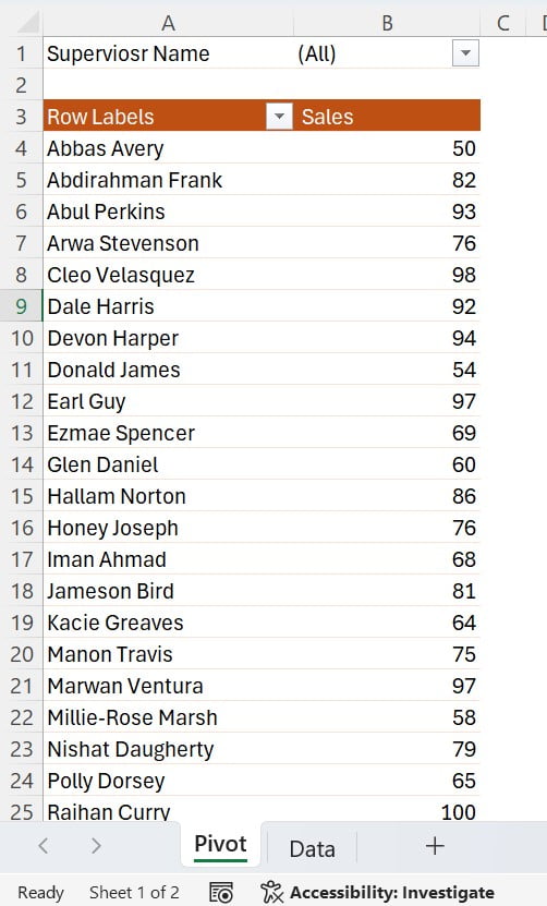
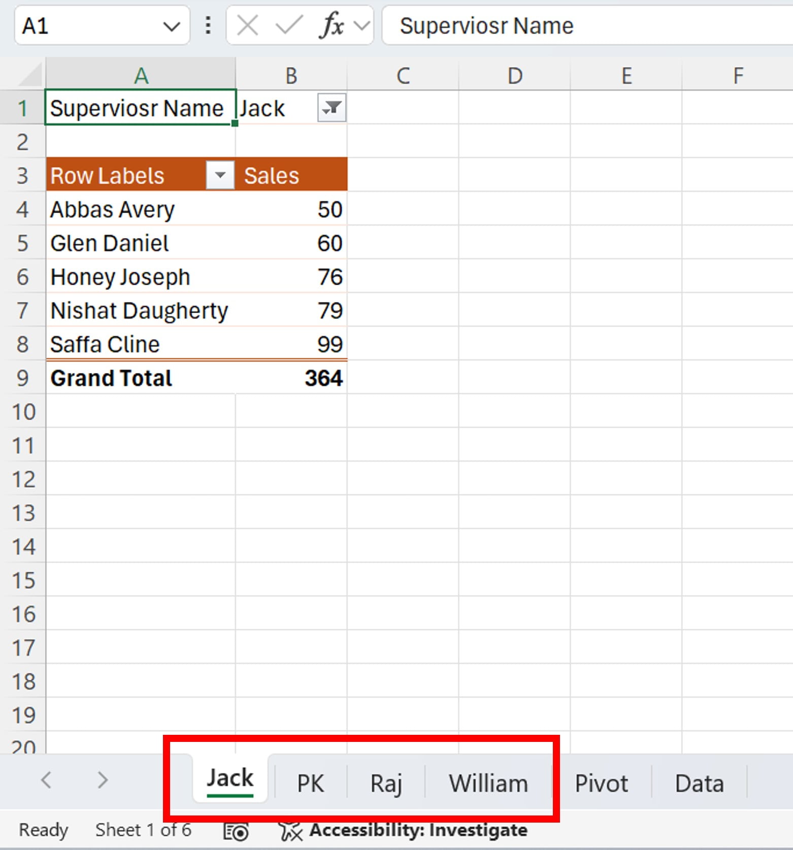
Before we get into the nitty-gritty, let’s set the stage. Imagine you have a primary pivot table in Excel. It’s structured with ‘Employee Name’ as rows, ‘Sales’ in values, and ‘Supervisor Name’ as a filter. Picture a scenario where you have four supervisors: PK, Raj, Jack, and William. The goal? To create a separate sheet for each supervisor, each containing a pivot table where the ‘Employee Name’ is in rows, ‘Sales’ is in values, and the respective ‘Supervisor Name’ is filtered. Sounds complicated? It’s simpler than you think!
Step-by-Step Guide: Creating Multiple Pivot Sheets
Now, let’s break down the process into easy, actionable steps:
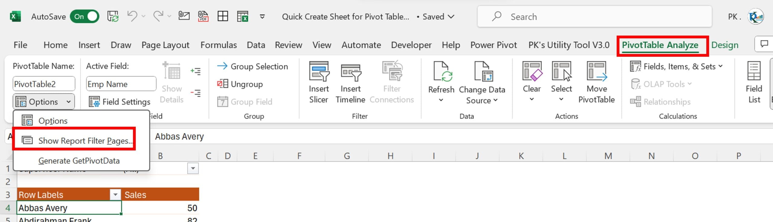
Step 1: Initiate the Pivot Table Analyze Feature
The journey begins with a simple click. Click anywhere on your main pivot table. This action brings up the ‘Pivot Table Analyze’ window in the Excel ribbon.
Step 2: Discover the ‘Options’
Next, navigate to the ‘Options’ drop-down. Here, click on the “Show Report Filter Pages” option. This is your key to automating the creation of multiple sheets.
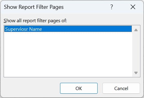
Step 3: Engage with the ‘Show Report Filter Pages’
Upon clicking “Show Report Filter Pages”, a popup window appears, showcasing a list of filters. This list is your pivot table’s way of asking, “What do you want to focus on?”
Step 4: Select Your Focus – The Supervisor Name
In this pivotal moment, select ‘Supervisor Name’ from the list. This choice tells Excel exactly what to filter in the new sheets.
Step 5: Witness the Magic
Now, the grand finale. Click ‘OK’, and watch as Excel performs its magic. In mere moments, multiple sheets spring to life, each named after a supervisor. Each sheet presents a pivot table filtered by that supervisor’s name. It’s efficiency and organization, all with a few clicks.
Embracing the Magic of Pivot Tables
Through these steps, what once seemed like a daunting task transforms into a straightforward, almost effortless process. Pivot tables are not just about data – they’re about unlocking potential, saving time, and enhancing your data analysis skills.
We hope this guide has illuminated the path to pivot table proficiency. Remember, the key to mastering Excel is practice, exploration, and a bit of magic – all of which you now possess.
Visit our YouTube channel to learn step-by-step video tutorials
Watch the step-by-step video tutorial:
Click here to download the practice file