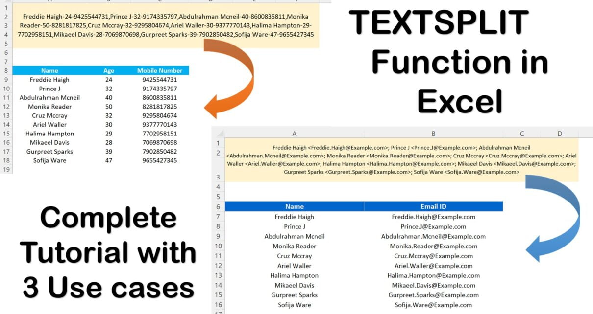
TEXTSPLIT is extremely useful function in Excel. We use it to split text by using column and row delimiters in Excel. This function can enable you to split the text across columns or down by rows. We will explain TEXTSPLIT function with 3 use cases in this blog post.
Syntax of the TEXTSPLIT function
Below is the syntax of TEXTSPLIT function in Excel
=TEXTSPLIT(text,col_delimiter,[row_delimiter],[ignore_empty], [match_mode], [pad_with])
Below are the explain of each parameter of TEXTSPLIT function
- text: Provide the reference for the text you want to split. It is required parameter.
- col_delimiter: The delimiter text that is the point where to spill the text across columns.
- row_delimiter: The delimiter text that is the point where to spill the text across rows. It is optional.
- ignore_empty: Select TRUE to ignore consecutive delimiters. Defaults value is FALSE to creates a blank cell. It is optional.
- match_mode: Select 1 to perform a case-insensitive match. Default value is 0, which is for a non-case-sensitive match. It is Optional.
- pad_with: Put the value with which to pad the result. The default value is #N/A, you can change it.
Here, we have explained the TEXTSPLIT Function with three Use Cases as given below
Use case 1:
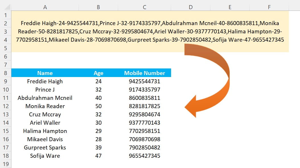
In the first use case we have a data of Name, Age and Mobile Number in combine format, and we have format it is using TEXTSPLIT function.
=TEXTSPLIT(A1,"-",",")
Use case 2:
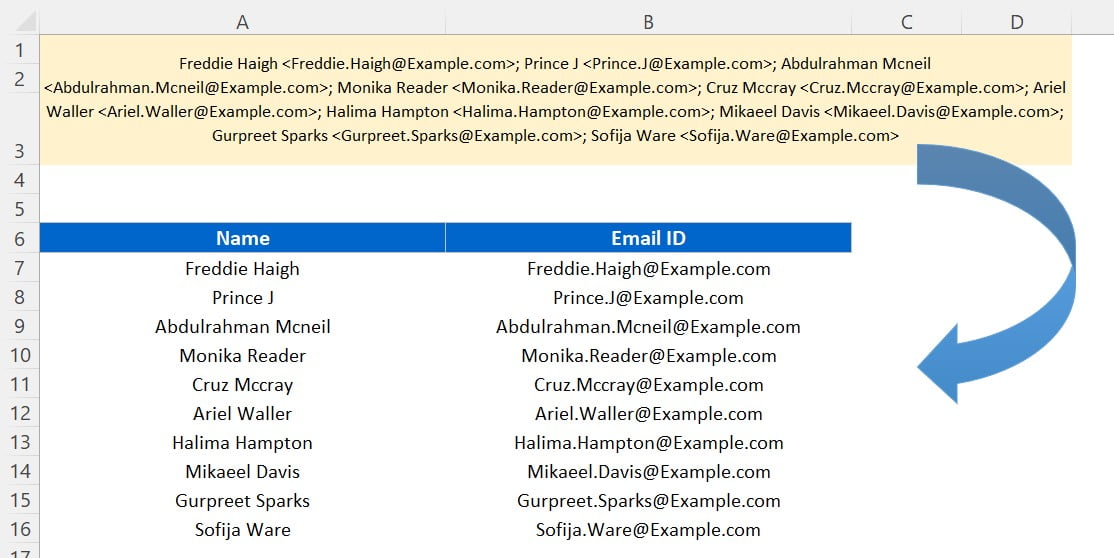
In the second use case we have multiple email ids and name which are copied from the outlook mail. We need to get the proper display name and email id in separate column.
=SUBSTITUTE(TEXTSPLIT(A1," <","; "),">","")
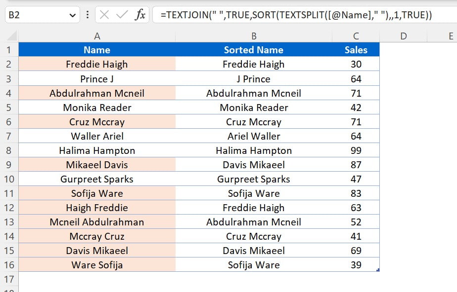
Use Case 3:
In the third use case, we have used the TEXTSPLIT function with some other functions to highlight the duplicate names even if first name and last name is shuffled.
To create the Sorted Name column, we have used below formula then we have conditional formatting on the Name column with the help of Sorted Name column.
=TEXTJOIN(" ",TRUE,SORT(TEXTSPLIT([@Name]," "),,1,TRUE))
Visit our YouTube channel to learn step-by-step video tutorials