VBA UserForm to Segregate Data into Multiple Worksheets

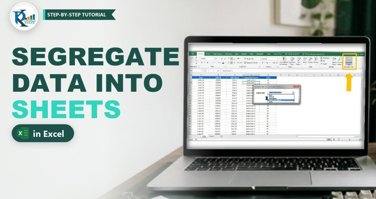
When you need to segregate data into multiple worksheets, one sheet per supervisor, per employee or per date, copying and filtering by hand takes ages and is easy to get wrong. In this tutorial you build PK’s VBA UserForm that does it in one click: pick any column header from a drop-down, click Run, and a new workbook appears with one worksheet for every unique value in that column. You will also store the macro in your Personal Macro Workbook and add a button for it to the Excel ribbon, so it works on the active sheet of any workbook you open.

Watch the Video Tutorial

PK demonstrates the form on sales data, builds it from an empty UserForm, fixes the date and number-format problems step by step, then adds the macro to the ribbon through the Personal Macro Workbook.

What You Will Build

• A UserForm with a Select Field drop-down and Run and Cancel buttons.
• A drop-down filled automatically with the headers in row 1 of the active sheet.
• A Run macro that creates a new workbook with one sheet per unique value, named after that value.
• Date and number handling, so it works on dates, IDs and text alike.
• A ribbon button that opens the form from any workbook.

The Sample Data

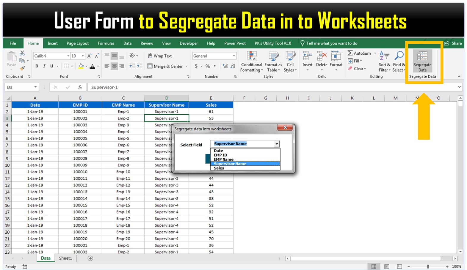
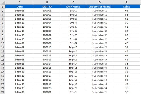
The data sits on the active sheet with headers in row 1: Date, EMP ID, EMP Name, Supervisor Name and Sales. There are 4 supervisors and 20 employees, with one row per sales record.

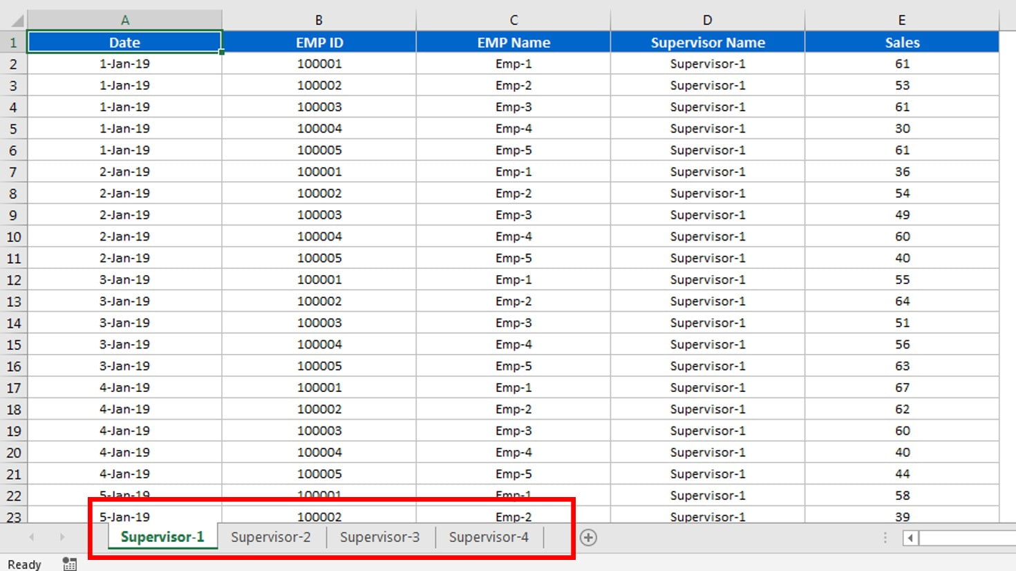
Segregating by Supervisor Name gives 4 sheets, by EMP Name 20 sheets, and by Date one sheet for each of the 31 dates. The original data is never changed: everything goes into a new workbook.

Part 1: Design the UserForm

Step 1: Insert the form

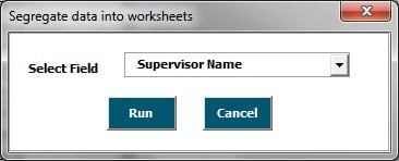
Open the Visual Basic Editor (Developer → Visual Basic or Alt+F11) and choose Insert → UserForm. In the Properties window give it a name and caption. PK names it myForm; the finished form’s caption is Segregate data into worksheets. Pick a white back colour or any colour you like.

Step 2: Add the label and the drop-down

From the Toolbox add a Label with the caption Select Field and make its font bold. Next to it add a ComboBox (ComboBox1) and make it wide enough for long header names.

Set the ComboBox Style property to fmStyleDropDownList. With the default combo style users could type any text; the drop-down list style lets them only pick a real header from the list.

Step 3: Add the Run and Cancel buttons

Add two CommandButtons. Set the caption of CommandButton1 to Run and of CommandButton2 to Cancel.

Part 2: The VBA Code Behind the Form

Step 4: Fill the drop-down when the form opens

Put Option Explicit as the very first line of the form’s code module, above every procedure. Then double-click the form, choose Initialize in the event list on the right, and add this code. It reads every header in row 1 of the active sheet into the ComboBox:

Private Sub UserForm_Initialize()

If Application.WorksheetFunction.CountA(ActiveSheet.Range("1:1")) > 0 Then
Dim i As Integer
For i = 1 To Application.WorksheetFunction.CountA(ActiveSheet.Range("1:1"))
If ActiveSheet.Cells(1, i).Value <> "" Then
Me.ComboBox1.AddItem ActiveSheet.Cells(1, i).Value
End If
Next i
End If

End Sub

The CountA check makes sure row 1 has at least one header, and the loop runs once per header. Because it always uses ActiveSheet, the form works on whatever sheet you are looking at.

Step 5: Close the form with Cancel

Private Sub CommandButton2_Click()
Unload Me
End Sub

Step 6: Segregate the data with Run

This is the main procedure from the original tutorial (paste it below the other procedures; Option Explicit is already at the top of the module):

Private Sub CommandButton1_Click()

Application.DisplayAlerts = False

Dim nwb As Workbook
Dim nsh As Worksheet
Dim dsh As Worksheet
Dim support As Worksheet

Set dsh = ActiveSheet

Dim col_number As Integer
Dim i As Integer

col_number = Application.WorksheetFunction.Match(Me.ComboBox1.Value, dsh.Range("1:1"), 0)

Set nwb = Workbooks.Add
Set support = nwb.Sheets(1)

dsh.AutoFilterMode = False
dsh.Cells(1, col_number).EntireColumn.Copy
support.Range("A1").PasteSpecial xlPasteValuesAndNumberFormats
support.UsedRange.RemoveDuplicates 1, xlYes

For i = 2 To Application.CountA(support.Range("A:A"))
Set nsh = nwb.Sheets.Add(after:=Sheets(Sheets.Count))
dsh.UsedRange.AutoFilter col_number, VBA.IIf(support.Range("A" & i).NumberFormat = "General", support.Range("A" & i).Value, VBA.Format(support.Range("A" & i).Value, support.Range("A" & i).NumberFormat))
dsh.UsedRange.Copy nsh.Range("A1")
On Error Resume Next
nsh.Name = VBA.IIf(support.Range("A" & i).NumberFormat = "General", support.Range("A" & i).Value, VBA.Format(support.Range("A" & i).Value, support.Range("A" & i).NumberFormat))
On Error GoTo 0

nsh.UsedRange.EntireColumn.ColumnWidth = 25
dsh.AutoFilterMode = False
ActiveWindow.DisplayGridlines = False
Next i

support.Delete

MsgBox "Process Completed"

End Sub

How the Segregate Code Works

1. Find the selected column

dsh remembers the data sheet before anything else changes. MATCH looks for the header you picked in row 1 and returns its position, for example 4 for Supervisor Name. That number is stored in col_number.

2. Build a list of unique values on a support sheet

Workbooks.Add creates the output workbook, and its first sheet becomes the support sheet. Any existing filter on the data is removed, the chosen column is copied and pasted as values and number formats, and RemoveDuplicates 1, xlYes leaves one row per unique value under the header. Keeping the number formats matters for the next step.

3. One loop pass per unique value

The loop starts at row 2 (row 1 is the header) and runs up to the number of filled cells in column A. For each value it:

• adds a sheet after the last sheet with after:=Sheets(Sheets.Count), so the sheets appear in the same order as the list (without it, new sheets are added in front and the order is reversed, as PK shows in the video);
• filters the data on col_number for that value and copies the visible rows, header included, to cell A1 of the new sheet;
• renames the sheet after the value, sets the column width to 25, removes the filter and hides gridlines.

4. Why IIf and Format are needed

When PK first ran the macro on Date, it failed: the filter needs the date as it is displayed, such as 1-Jan-19. So the value is converted with VBA.Format(value, NumberFormat). But then EMP ID failed, because its format is General, which is not a real format code. VBA.IIf solves both: if the cell’s format is General, use the value as it is; otherwise format it with the cell’s own number format. The same expression is used for the filter criteria and for the sheet name.

5. Tidy up

Some formatted dates contain characters that are not allowed in a sheet name, so the rename sits between On Error Resume Next and On Error GoTo 0; if it fails, the sheet keeps Excel’s default name. After the loop the support sheet is deleted. Application.DisplayAlerts = False at the top stops Excel from asking you to confirm that delete. Finally, a message says Process Completed.

Part 3: Run It from the Ribbon

Step 7: Add a macro that shows the form

Insert a standard module and add a short macro that shows the form modeless (myForm.Show False). In the video the module is renamed Call_My_From_Module and the macro is Call_My_From:

Sub Call_My_From()
    myForm.Show False   'False = modeless: you can still click the sheet
End Sub

Step 8: Move the form and module to PERSONAL.XLSB

To use the tool in every workbook, it must live in your Personal Macro Workbook. If you do not have one yet, go to View or Developer → Record Macro, choose Store macro in: Personal Macro Workbook, click OK and stop recording straight away. PERSONAL.XLSB now appears in the Visual Basic Editor. Drag the form and the module into it, then click any module of PERSONAL.XLSB and save.

Step 9: Add a button to the ribbon

1. Right-click the ribbon and choose Customize the Ribbon.
2. On the right, expand a tab (in the video PK expands the Data tab and adds the group after the Outline group; the screenshot above shows it on the Home tab, and any tab works), click New Group and Rename it Segregate Data.
3. In Choose commands from select Macros, pick PERSONAL.XLSB!Call_My_From and click Add.
4. Rename the button Segregate data into worksheets, choose an icon and click OK.

The button now opens the form in any workbook. Select the sheet with your data, click it, pick a field and click Run.

Need the sheets back in one table? In the video PK uses the worksheet manager of his free PK’s Utility Tool V1.0 to consolidate selected sheets, which also adds a column with the source sheet name.

Common Errors and Fixes

The errors, tips and alternative below are additions from general VBA practice; they are not covered in the video.

Run-time error 1004 when you click Run without a field

MATCH cannot find an empty value. Add a check at the start of the Run procedure: if Me.ComboBox1.ListIndex = -1, show a message and Exit Sub.

Some sheets are called Sheet2, Sheet3 and so on

The value could not be used as a sheet name: it is longer than 31 characters, contains one of : \ / ? * [ ], or matches another name. The data is still correct; rename the sheet by hand or clean the values first.

Rows are missing or the wrong columns are copied

The code uses UsedRange and expects headers in row 1. Remove blank rows and titles above the table, and fill any blank cells in the column you segregate by.

Tips

• Save the output workbook straight away; it is new and unsaved when the macro finishes.
• Turn on Application.ScreenUpdating = False at the start for a faster run on large data.
• For a quick summary per value instead of raw rows, a PivotTable’s Show Report Filter Pages option also creates one sheet per item.
• Microsoft explains the filter arguments in the Range.AutoFilter method reference.

Want It Ready-Made?

The finished VBA User form for Segregate data into multiple worksheets is available on NextGenTemplates.com with the form and code from this tutorial ready to use. For more automation templates, browse the Excel VBA tools collection.

Related Tutorials

• Split Data into Separate Workbooks in Excel (VBA Macro)
• Macro to Create Multiple Worksheets from a Selection
• Personal Macro in Excel: Quick Data Formatting with Ctrl+M
• VBA Multilevel Dependent Drop-Down in a UserForm
• Excel FILTER Function: Syntax, Multiple Criteria and Examples

Frequently Asked Questions

How do I split Excel data into multiple worksheets automatically?

Use a macro that lists the unique values of a column, then filters the data for each value and copies it to its own sheet. The UserForm in this tutorial does that for any column you pick.

Does the macro change my original data?

No. It only filters the source sheet temporarily and removes the filter again. All new sheets are created in a new workbook.

Why does the code use IIf and Format for the filter value?

Dates must be filtered as they are displayed, so they are formatted with the cell’s own number format. Values in General format are used as they are, because General is not a format code.

How can I use the form in every workbook?

Move the form and its macro into your Personal Macro Workbook, PERSONAL.XLSB, and add the macro to the ribbon with Customize the Ribbon.

Can I stop users from typing in the drop-down?

Yes. Set the ComboBox Style property to fmStyleDropDownList, so only existing headers can be selected.

About the Author

PK is a Microsoft Excel expert and trainer and the founder of PK: An Excel Expert and NextGenTemplates.com. He has been teaching Excel, VBA, Power Query and Power BI since 2016 on his YouTube channel.

Conclusion

With one UserForm and about 40 lines of VBA you can segregate data into multiple worksheets by any column: the form lists the headers, MATCH finds the column, a support sheet holds the unique values, and AutoFilter copies each group to its own sheet in a new workbook. Store it in PERSONAL.XLSB, add a ribbon button, and splitting a report by supervisor, employee or date becomes a two-click job.