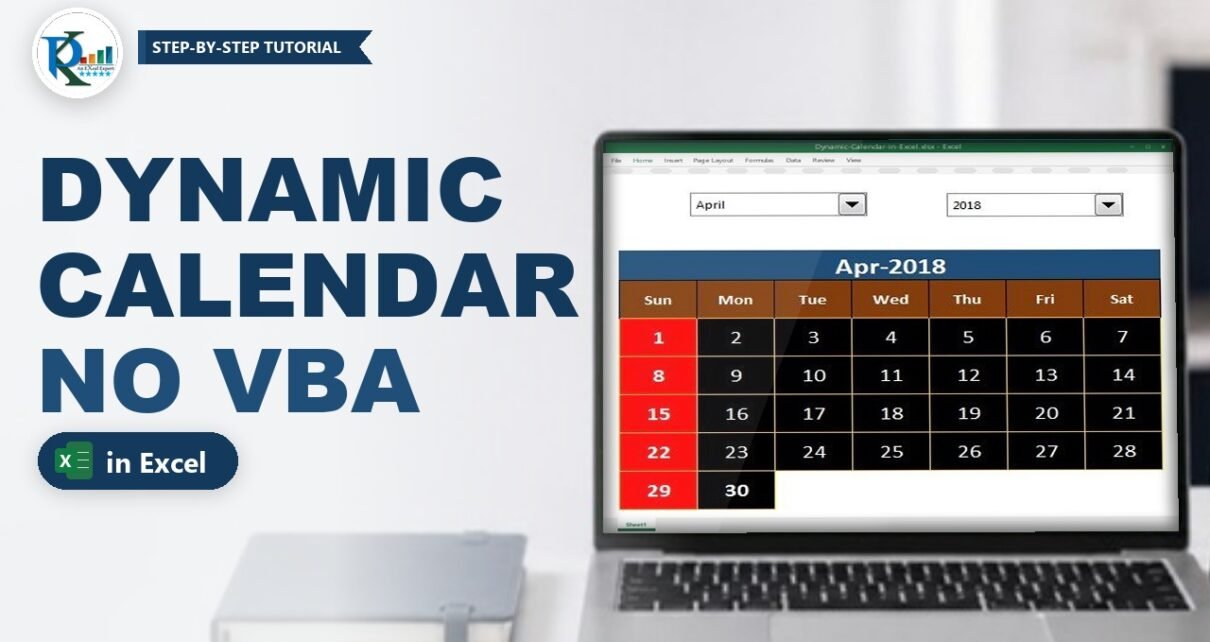
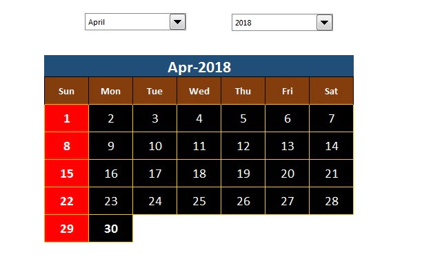
A dynamic calendar in Excel redraws itself the moment you pick a different month or year, so you never have to retype dates or shift cells around again. In this tutorial you build one with formulas and conditional formatting only – no VBA. Two Form Control combo boxes choose the month and the year, WEEKDAY puts day 1 under the right weekday, EOMONTH stops the grid at the last day of the month, and Sundays light up in red. It works in Excel 2010, 2013, 2016, 2019, 2021 and Microsoft 365.
⬇️ Download the Dynamic Calendar
Single-sheet workbook · .xlsx (no macros) · Excel 2010 and later
Watch the Video Tutorial
The video builds the same calendar from a blank sheet: the two combo boxes, the month header, the first-week formula, the remaining weeks and the conditional formatting that colours the grid.
What You Will Build
- Month and year drop-downs made with Form Control combo boxes (years 2000 to 2030).
- A live header that shows the selected month, for example Apr-2018.
- A 6 x 7 date grid (Sunday to Saturday) where day 1 always lands under the correct weekday.
- Automatic month length – 28, 29, 30 or 31 days, leap years included, with no blank-cell clean-up.
- Conditional formatting that paints Sundays red and formats only the cells that hold a date.
How the Workbook Is Laid Out
Everything sits on one sheet. A few helper cells do the work in the background and are hidden from view:
- P1:P12 – the month names January to December.
- Q1:Q31 – the years 2000 to 2030.
- A1 and A2 – the cell links of the two combo boxes (column A is hidden).
- B1 and B2 – the selected month name and year.
- C7:I7 (merged) – the month header; C8:I8 – Sun to Sat; C9:I14 – the date grid.
Gridlines and row/column headings are switched off in the View tab, so the sheet looks like a clean calendar card.
Part 1 – Month and Year Drop-Downs
Step 1: Type the lists
Type January to December in P1:P12 and the years 2000 to 2030 in Q1:Q31 (type 2000 and 2001, select both and drag the fill handle down).
Step 2: Insert the two combo boxes
Go to Developer › Insert › Combo Box (Form Control) and draw one above the calendar. Right-click it, choose Format Control and set:
- Month combo: Input range
$P$1:$P$12, Cell link$A$1, Drop down lines 12. - Year combo: Input range
$Q$1:$Q$31, Cell link$A$2, Drop down lines 20.
If you do not see the Developer tab, turn it on in File › Options › Customize Ribbon.
Step 3: Turn the positions into a month and a year
A combo box does not return the item you pick – it returns its position in the list. Pick April and A1 shows 4; pick 2018 and A2 shows 19. INDEX turns those positions back into real values:
B1  =INDEX(P:P,A1)
B2  =INDEX(Q:Q,A2)
With April and 2018 selected, B1 returns April and B2 returns 2018.
Part 2 – The Month Header
Step 4: Build the first day of the month
Merge C7:I7 and enter:
C7 =DATEVALUE("1-"&B1&"-"&B2)The formula joins the text 1-April-2018 and DATEVALUE converts it into a real Excel date. Give C7 the custom number format mmm-yyyy so it displays Apr-2018. This cell is the anchor for every other formula, so all the grid formulas point to $C$7 with absolute references. (If DATEVALUE gives you trouble on your PC, see the Common errors section for a locale-proof version.)
Type Sun, Mon, Tue, Wed, Thu, Fri and Sat in C8:I8.
Part 3 – The Dynamic Calendar Date Grid
Step 5: The first week (row 9)
The first row is the clever part. Day 1 has to appear under the right weekday and every cell before it must stay blank. In C9 enter:
C9 =IF(WEEKDAY($C$7)=COLUMNS($C$8:C8),$C$7,"")Then in D9 enter the version that also continues the count, and copy it across to I9:
D9 =IF(C9<>"",C9+1,IF(WEEKDAY($C$7)=COLUMNS($C$8:D8),$C$7,""))How the formula works
- WEEKDAY
($C$7)returns the day number of the 1st of the month: 1 for Sunday up to 7 for Saturday. April 1, 2018 was a Sunday, so it returns 1. COLUMNS($C$8:C8)counts the columns from C to the current column: 1 in column C, 2 in D, up to 7 in I. Because only the first part is locked, the count grows as you copy the formula right. In other words, it is the weekday number of that column.- When the two numbers match, the cell is where the month starts, so it shows
$C$7(the 1st). IF(C9<>"",C9+1,...)in D9 to I9 says: if the cell on my left already has a date, I am simply the next day. That is how the rest of the first week fills in.- Cells before the 1st return
""and stay empty.
Step 6: Weeks two to four (rows 10 to 12)
These rows can never be empty, so plain addition is enough:
C10  =I9+1
D10  =C10+1
Copy D10 across to I10, then copy C10:I10 down to row 12. Each row starts the day after the previous Saturday.
Step 7: Weeks five and six (rows 13 and 14)
Here the month can end, so each cell checks the last day of the month with EOMONTH before it adds a day:
C13  =IF(EOMONTH($C$7,0)>I12,I12+1,"")
D13  =IF(EOMONTH($C$7,0)>C13,C13+1,"")
Copy D13 to I13. In row 14 use the same pattern, with C14 pointing to I13: =IF(EOMONTH($C$7,0)>I13,I13+1,""). EOMONTH($C$7,0) returns the last date of the selected month (30-Apr-2018 here). As long as the previous cell is earlier than that date, the next day is shown; after the last day, cells return blank. Once a cell is blank, every cell after it compares the month end with text, which is FALSE, so they stay blank too.
Six rows are enough for any month: even a 31-day month that starts on a Friday or Saturday fits.
Step 8: Show only the day number
The grid holds full dates. Select C9:I14 and apply the custom number format d so each cell shows just 1, 2, 3 and so on. Keeping real dates (rather than plain numbers) is what makes the highlights and any later lookups possible.
Part 4 – Conditional Formatting
The workbook uses two rules, both based on the formula LEN(TRIM(cell))>0, which means "this cell is not blank":
- Sundays – applied to C9:C14 with
=LEN(TRIM(C9))>0: red fill, bold white font and a thin gold border. - Weeks five and six – applied to C13:I14 with
=LEN(TRIM(C13))>0: black fill, bold white font and the same gold border, so the last row only shows boxes for real days and the grid ends cleanly.
Create each rule with Home › Conditional Formatting › New Rule › Use a formula to determine which cells to format. Keep the reference relative (no $ signs) so it moves with each cell. The Sunday rule sits at the top of the list, so it wins where the two ranges overlap.
Modern Excel Alternative (Microsoft 365 and Excel 2021)
If you have dynamic arrays, you can replace the whole grid with a single formula in C9 (leave C9:I14 empty so it can spill):
=LET(f,DATE(B2,A1,1),s,f-WEEKDAY(f)+1,d,SEQUENCE(6,7,s),IF(MONTH(d)=A1,d,""))fis the 1st of the month. DATE uses the combo box positions directly, because A1 already holds the month number.ssteps back to the Sunday on or before the 1st.SEQUENCE(6,7,s)creates 42 consecutive dates in a 6 x 7 block.IF(MONTH(d)=A1,d,"")blanks out days from the previous and next month.
Apply the d number format and the same conditional formatting rules. The classic formulas above still work in every version, so use whichever fits your Excel.
Common Errors and Fixes
#VALUE! in the month header
DATEVALUE reads text according to your Windows regional settings and language, so 1-April-2018 may not be recognised on every PC. Replace C7 with =DATE(B2,A1,1), which builds the date from numbers and works everywhere.
The grid shows numbers like 43191
Those are dates without a date format. Select C9:I14 and apply the custom format d.
Changing the drop-down does nothing
Right-click the combo box, open Format Control and check the cell link. If it is empty or points to the wrong cell, A1/A2 never change and neither does the calendar.
#SPILL! with the SEQUENCE version
Something is typed in C9:I14. Clear the block so the 42 dates have room to spill.
Tips
- Want Monday as the first column? Change the headers to Mon-Sun and use
WEEKDAY($C$7,2), which numbers Monday as 1. Move the Sunday highlight rule to column I. - Highlight today with one more rule on C9:I14:
=C9=TODAY(). - Extend the year list in column Q and update the year combo’s input range to match.
- Hide the helper columns and turn off gridlines so users only see the calendar and the two drop-downs.
- Microsoft’s guide to conditional formatting in Excel covers formula-based rules in detail.
Want It Ready-Made?
If you need finished calendars and planners rather than building them, the Calendar & Planner Pack on NextGenTemplates.com bundles 12 Excel and Google Sheets templates, or you can browse all Excel templates. To master WEEKDAY, EOMONTH, INDEX, SEQUENCE and the other date formulas step by step, join the video course Excel + AI Mastery: 100 Essential Formulas and Real-World Projects.
Related Tutorials
- Excel Form Controls: Combo Box, Spin Button and Option Buttons
- Highlight Dates in Excel: Due Today, Overdue, This Week and Weekends
- SEQUENCE Function in Excel with Example
- Excel DATEVALUE Function: Convert Text to Dates
- Student Attendance Calendar in Excel
Frequently Asked Questions
How do I make a calendar in Excel that changes with the month?
Build the 1st of the selected month in one cell, then let every grid cell calculate from it. In this template C7 holds the 1st, WEEKDAY places it under the right weekday, each following cell adds 1, and EOMONTH stops the grid at the month end.
Do I need VBA to create a dynamic calendar in Excel?
No. The calendar uses Form Control combo boxes, formulas and conditional formatting only. The file is a normal .xlsx with no macros.
Why does my combo box return a number instead of the month name?
A Form Control combo box always returns the position of the selected item. Use INDEX on the list, for example =INDEX(P:P,A1), to get the month name back.
How do I start the calendar week on Monday?
Change the weekday headers to Mon to Sun and use WEEKDAY($C$7,2) in the first-week formulas. With return type 2, Monday is 1 and Sunday is 7, which matches the new column order.
Does the calendar handle leap years?
Yes. EOMONTH returns the real last day of the month, so February shows 29 days in a leap year and 28 otherwise.
Can I build it with a single formula?
Yes, in Excel 2021 or Microsoft 365. The LET and SEQUENCE formula in the Modern Excel Alternative section builds 42 dates from the Sunday before the 1st and blanks out the days of other months, so the whole 6 x 7 grid spills from one cell.
About the Author
PK is a Microsoft Excel expert and trainer and the founder of PK: An Excel Expert and NextGenTemplates.com. He has been teaching Excel, Power Query and Power BI since 2016 on his YouTube channel.
Conclusion
A dynamic calendar in Excel needs just a handful of formulas: INDEX to read the drop-downs, WEEKDAY to place the 1st, simple addition for the middle weeks and EOMONTH to end the month. Add two conditional formatting rules and you have a clean, reusable calendar that updates with one click. Download the file, pick a month and see it redraw itself.