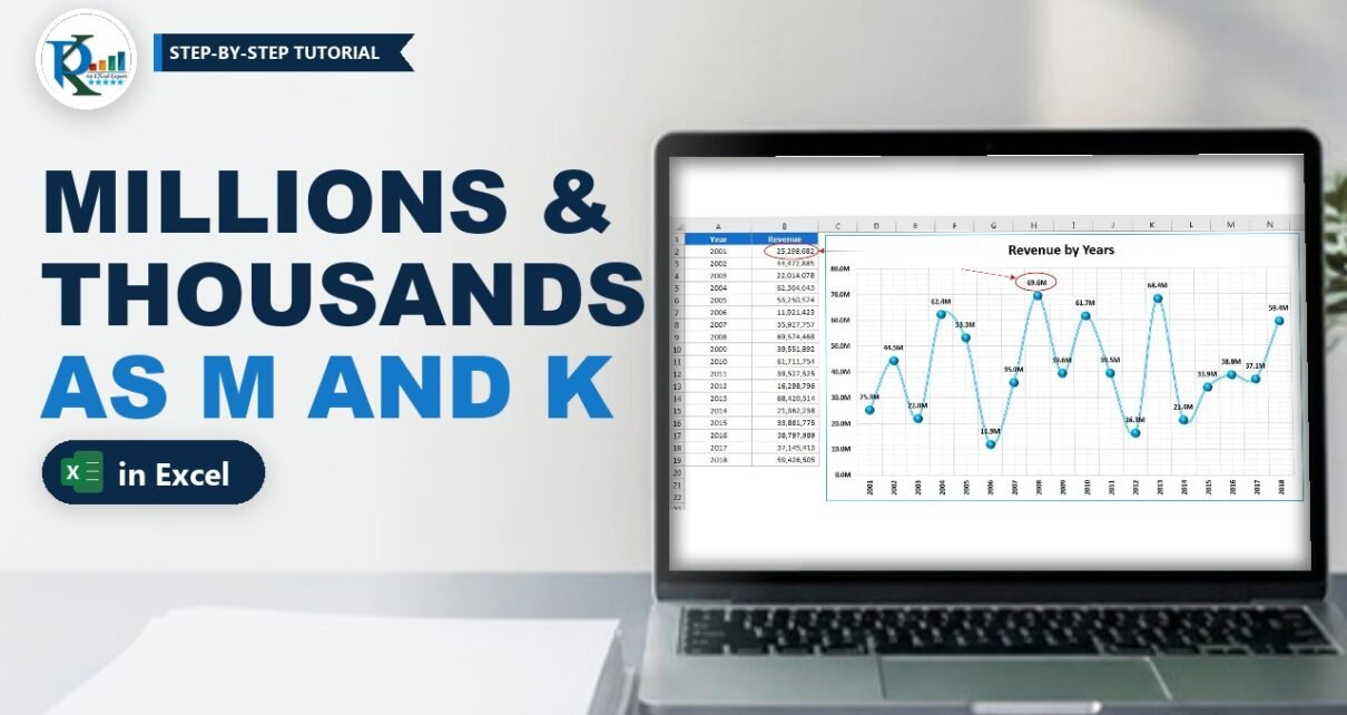
A dynamic number format in Excel shows big numbers as 1.2K or 3.5M automatically, so your tables and charts stay readable without changing a single value. In this tutorial you will format a revenue chart in millions (data labels and the vertical axis), learn the thousand and million custom codes, and then combine them into one conditional format that picks K or M by itself. No VBA and no helper columns: just custom number formats, which work in every version of Excel from 2007 to Microsoft 365.
⬇️ Download the Practice File
Two sheets (chart + sales summary) · .xlsx (no macros) · Excel 2007 and later
Watch the Video Tutorial
In the video PK fixes an unreadable revenue chart, builds the thousand and million formats on a test cell, and finishes with the one conditional format that switches between K and M on its own.
What You Will Build
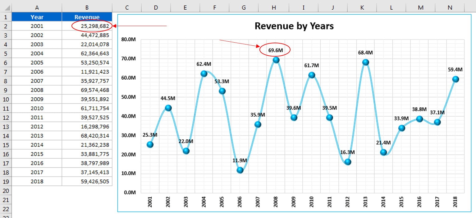
- A readable revenue chart whose data labels show values like 62.4M instead of 62,364,643.
- A matching vertical axis that reads 10.0M, 20.0M, 30.0M and so on.
- A thousands format (
0.0,"K") and a millions format (0.0,,"M") you can reuse anywhere. - One dynamic format that shows M for millions, K for thousands and the plain number below 1,000.
- A table where the real values stay untouched, so SUM, lookups and pivots still calculate on the full numbers.
How the Practice File Is Laid Out
- Sheet1: Year in A2:A19 (2001 to 2018) and Revenue in B2:B19. Revenue uses
=RANDBETWEEN(10000000,70000000), so every value is between 10 and 70 million. The line chart Revenue by Years sits next to it. - Sheet2: a Sales Summary table in D3:F13 with Product-1 to Product-10, Unit Sold (
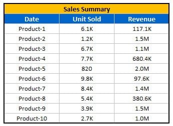
=RANDBETWEEN(500,10000)) and Revenue (=RANDBETWEEN(10000,2000000)). E4:F13 carry the dynamic K/M format.
Because the numbers come from RANDBETWEEN, press F9 to recalculate and watch the format switch between K and M as the values change.
Part 1 – Show Millions on an Excel Chart
Step 1: Insert the line chart and fix the years
Select A1:B19 and go to Insert › Line Chart. Because the years are numbers, Excel plots them as a second series instead of using them as the horizontal axis. Fix it in two clicks:
- Right-click the chart and choose Select Data.
- Select the Year series and click Remove.
- Under Horizontal (Category) Axis Labels click Edit and select A2:A19.
Now the years run along the bottom and only Revenue is plotted.
Step 2: Add data labels (and see the problem)
Add data labels and set the position to Above. You get labels like 68,197,523 on every point. They overlap and nobody can read them at a glance. Shortening them to millions is the fix.
Step 3: The quick way – Display units
Right-click the vertical axis, choose Format Axis and look for Display units. Pick Hundreds, Thousands or Millions and Excel divides the axis for you, with an optional Millions label on the side. It works, but the numbers show as 10, 20, 30 with no M after them, so a reader has to look for the side label to know the unit. A custom number format puts the M on every number, which is why it is the better option.
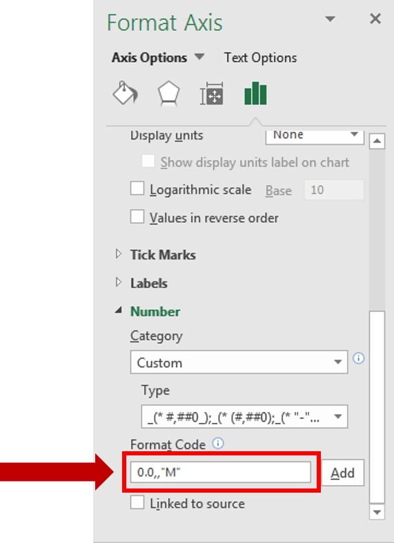
Step 4: Format the vertical axis in millions
- In Format Axis, set Display units back to None.
- Open the Number section and make sure the category is Custom.
- In Format Code type
0.0,,"M"and click Add.
Step 5: Format the data labels in millions
Right-click any data label, choose Format Data Labels, scroll down to Number, paste the same 0.0,,"M" into Format Code and click Add. Every label now reads like 44.5M or 69.6M.
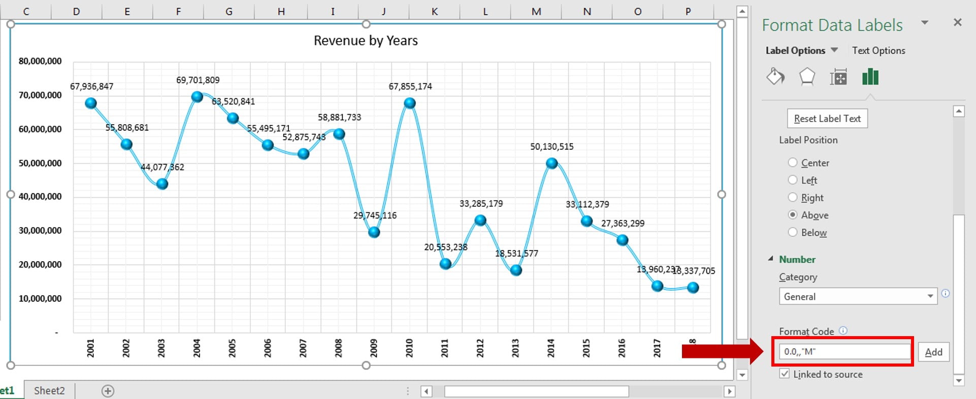
Look at the sheet: B2 still shows 25,298,682. A number format only changes how a value is displayed, never the value itself.
Part 2 – Custom Formats for Thousands and Millions
Before making the format dynamic, it helps to understand the two building blocks. Test them on a spare cell.
Step 6: The thousands format
Type 1234 in a cell. Press Ctrl+1 (or right-click › Format Cells), choose Custom and type this in the Type box:
0.0,"K"The cell shows 1.2K, while the formula bar still says 1234.
Step 7: 0.0 versus #.0
You can also write the code as #.0,"K". The difference shows with small numbers: 650 displays as 0.7K with 0.0 but as .7K with #.0. A 0 forces a digit before the decimal point; a # shows one only when it is needed. For reports, 0.0 reads better.
Step 8: The millions format
A million is a thousand thousands, so you use two commas. Type 1234567 in a cell and apply:
0.0,,"M"The cell shows 1.2M. This is exactly the code you used on the chart in Part 1.
How the format code works
0.0shows one decimal place, with at least one digit before the point.- Each
,placed after the last digit placeholder divides the displayed value by 1,000. One comma = thousands, two commas = millions. "K"or"M"is literal text added after the number. Anything in double quotes is printed as it is.
Part 3 – Dynamic Number Format in Excel for K and M
Step 9: Write the conditional format
Now combine both codes. Select E4:F13 on Sheet2, press Ctrl+1, choose Custom and type:
[>=1000000]0.0,,"M";[>=1000]0.0,"K";0Click OK. Revenue now shows values like 1.5M and 680.4K side by side, and Unit Sold shows 6.1K or 820, all from one format.
How the dynamic format works
With conditions, a custom format uses up to three number sections separated by semicolons, and only the first two can carry a condition in square brackets. Excel reads them left to right:
[>=1000000]0.0,,"M"– if the value is 1,000,000 or more, divide by a million and add M.[>=1000]0.0,"K"– otherwise, if it is 1,000 or more, divide by a thousand and add K.0– everything else shows as a plain whole number, so 820 stays 820.
Press F9 a few times. As RANDBETWEEN produces new numbers, each cell switches between M, K and plain digits on its own.
Step 10: Use it on the chart too
If your chart mixes small and large values, paste the same dynamic code into Format Data Labels › Number › Format Code or Format Axis › Number and click Add. Labels under a million then show K, and larger ones show M.
Common Errors and Fixes
The cells show odd values like 9801.0K
You typed a comma instead of a semicolon between two sections. That happens in the video too: with a comma, Excel reads it as part of the number pattern and the result is wrong. Check that the sections are separated by ; exactly as in Step 9.
The chart labels did not change
You typed the code but did not click Add, or you edited the wrong element. The axis and the data labels each need their own format. When you click Add, Linked to source switches off, so the chart stops copying the sheet format.
Display units shows numbers without M
That is how Display units works. Set it back to None before applying the custom code, otherwise Excel divides twice and you see 0.0M everywhere.
Negative numbers are not shortened (addition)
The conditions only test for values above 1,000 or 1,000,000, so a negative value falls through to the last section and shows in full. If your data has negatives, use a separate format or the TEXT approach in the Tips below.
Tips
- Billions (addition): Excel allows only two conditions per format, so swap the plain section for thousands:
[>=1000000000]0.0,,,"B";[>=1000000]0.0,,"M";0.0,"K". Values under 1,000 then show as 0.x K. - Need it as text in a title or a label? (addition): the TEXT function accepts the same code, for example
=TEXT(B2,"0.0,,""M"""), with the inner quotes doubled. - Regional settings (addition): the scaling commas follow your Windows thousands separator. If your PC uses a dot or a space as the separator, use that character instead of the comma.
- The custom format is saved in the workbook, so after the first time you can pick it from the Custom list instead of typing it again.
- Microsoft’s guidelines for customizing a number format explain sections, conditions and scaling commas in full.
Want It Ready-Made?
If you would rather start from finished, professionally formatted charts, the Chart Templates in Excel pack on NextGenTemplates.com gives you ready chart layouts to drop your data into, and you can browse the full Charts and Visualization templates. To learn charts, slicers and dashboard formatting step by step, join the video course Excel Pivot Tables and Dashboards.
Related Tutorials
- Highlight Sales Figures with Custom Number Formatting in Excel
- Arrow Symbols in Excel with Custom Formatting and Data Bars
- Conditional Formatting in a Line Chart in Excel: Green vs Red
- Highlight a Data Point in an Excel Line Chart Dynamically
- Advanced Excel Charts and Infographics
Frequently Asked Questions
How do I show numbers in millions in Excel?
Open Format Cells with Ctrl+1, choose Custom and use a zero, a decimal point, a zero, two commas and the letter M in quotes. Step 8 shows the exact code. Each comma after the digits divides the display by 1,000, so two commas give millions.
Does a custom number format change the actual value?
No. It only changes what you see. The formula bar still shows the full number, and every formula, pivot table and chart uses the full value.
How do I format chart data labels in thousands or millions?
Right-click a data label, choose Format Data Labels, open Number, type the custom code in Format Code and click Add. Do the same for the vertical axis in Format Axis.
Can one format show both K and M automatically?
Yes. Put a condition in square brackets in front of each section: one for values of a million or more, one for values of a thousand or more, and a plain section for the rest. Step 9 shows the full code.
Why does Display units not show an M after the number?
Display units divides the axis and can add a Millions label beside it, but it does not add a suffix to each number. Set it to None and use a custom format if you want 10.0M on every tick.
Can I add billions to the dynamic format?
Yes, but a custom format allows only two conditions. Use one condition for billions with three commas, one for millions with two commas, and let the last section handle thousands, as shown in the Tips.
About the Author
PK is a Microsoft Excel expert and trainer and the founder of PK: An Excel Expert and NextGenTemplates.com. He has been teaching Excel, Power Query and Power BI since 2016 on his YouTube channel.
Conclusion
A dynamic number format in Excel is one of those small tricks you will use in every report. Two commas and an M make a chart readable in seconds, and one conditional code with two sections lets Excel choose between K and M on its own, while the real values stay untouched underneath. Download the practice file, press F9 a few times and watch the format adapt.