Introduction
Are you ready to take your understanding of sales data to the next level? Our recent YouTube video, “Extract Unique Locations and Calculate Total Sales” does just that. It’s not just about numbers; it’s about making those numbers work for you. In this blog post, we’ll recap the essential lessons from the video, breaking down complex formulas into bite-sized, easy-to-understand insights.
Understanding the Data Structure
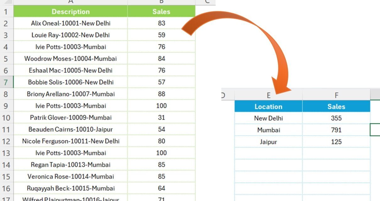
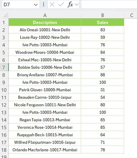
Before diving into the formulas, let’s clarify the data we’re dealing with. Imagine a spreadsheet filled with sales information. Column A contains a string of data representing the “Employee Name-Employee ID-Location” like “Alix Oneal-10001-New Delhi.” Column B is where the sales figures live, showing the sales amount corresponding to each employee’s description.
Extract Unique Locations and Calculate Total Sales
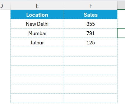
Our journey begins with the quest to identify unique locations from our list. The formula “=UNIQUE(TEXTAFTER(A2:A18,”-“,-1))” is our guiding light here. Let’s break it down:
UNIQUE(): This function is like a gatekeeper, ensuring that only one of each item passes through, giving us a list devoid of any duplicates.
TEXTAFTER(): Think of this as a skilled craftsman, carving out the part of the text after a specific delimiter. In our case, it slices right after the last hyphen “-“, giving us the precious location data.
By combining these two, we extract a pristine list of unique locations from our otherwise jumbled data.
Summing Up Sales: Deciphering “=SUMIF(A2:A18,”*”&E2#,B2:B18)”
Next, we turn our attention to summing up the sales for each location. This is where “=SUMIF(A2:A18,”*”&E2#,B2:B18)” comes into play. Here’s the breakdown:
SUMIF(): SUMIF function will adding up numbers but only the ones that meet a specific condition.
A2:A18: This is our range, the realm within which our accountant operates.
“*”&E2#: The condition here is a bit like a password. It says, “Add up the sales only if the location matches what’s listed in our unique locations list (E2#).”
B2:B18: These are the numbers our accountant is adding up – the sales figures.
In essence, this formula is tallying the sales for each unique location, giving us a clear view of where our numbers are coming from.
Conclusion
By demystifying these formulas, we’ve turned complex data into a clear, actionable format. Whether you’re a seasoned data analyst or a curious beginner, understanding these techniques is a powerful step towards making informed decisions and strategies. Remember, it’s not just about the numbers; it’s about the stories they tell and the decisions they inform. So, dive into your data, and let’s turn those insights into action!
Visit our YouTube channel to learn step-by-step video tutorials