Forecasting in Excel using linear regression lets you turn a few months of history into a day-by-day forecast with nothing more than built-in formulas and a chart trendline. In this tutorial you take 90 days of sales (1 January to 31 March 2019) and predict every day of April 2019 in four different ways: the FORECAST function, the TREND function, the SLOPE and INTERCEPT equation, and the equation Excel prints on a chart. All four give practically the same answer, and you will see exactly why.
⬇️ Download the Forecasting Practice File
Two-sheet workbook · .xlsx (no macros) · 90 days of sales plus all four forecast methods
Watch the Video Tutorial
In the video PK plots the sales on a chart, adds the linear trendline with its equation and R-squared, then fills the April forecast with FORECAST, TREND, SLOPE/INTERCEPT and the chart equation.
What You Will Build
- A scatter chart of daily sales with a linear regression trendline.
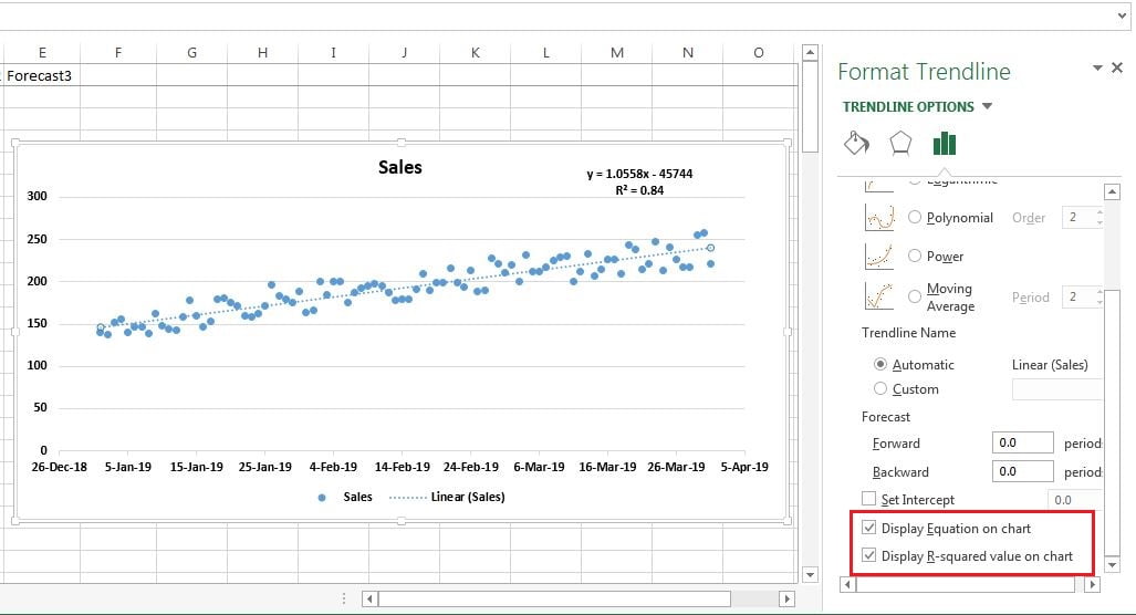
- The regression equation and R-squared displayed on the chart (y = 1.0558x – 45744, R² = 0.84).
- Four forecast columns for 1 to 30 April 2019, one per method.
- A line chart that shows actual sales and the forecast side by side.
How the Workbook Is Laid Out
- A2:A91 – dates from 1-Jan-2019 to 31-Mar-2019 (90 days).
- B2:B91 – daily sales, from 137 to 258 units.
- A92:A121 – the 30 April dates you want to predict. Column B stays empty here.
- C92:F121 – one column per forecast method (Forecast1 to Forecast4).
To create the April dates, type 1-Apr-19 in A92 and drag the fill handle down to A121.
Part 1 – Linear Regression with an Excel Chart
Step 1: Plot the actual sales
Select A1:B91 and go to Insert → Charts. A scatter chart works best (a line chart also works). In this data the dots rise in a steady pattern with no outliers. A straight-line forecast only makes sense when the history follows a roughly straight trend like this.
Step 2: Add a linear trendline
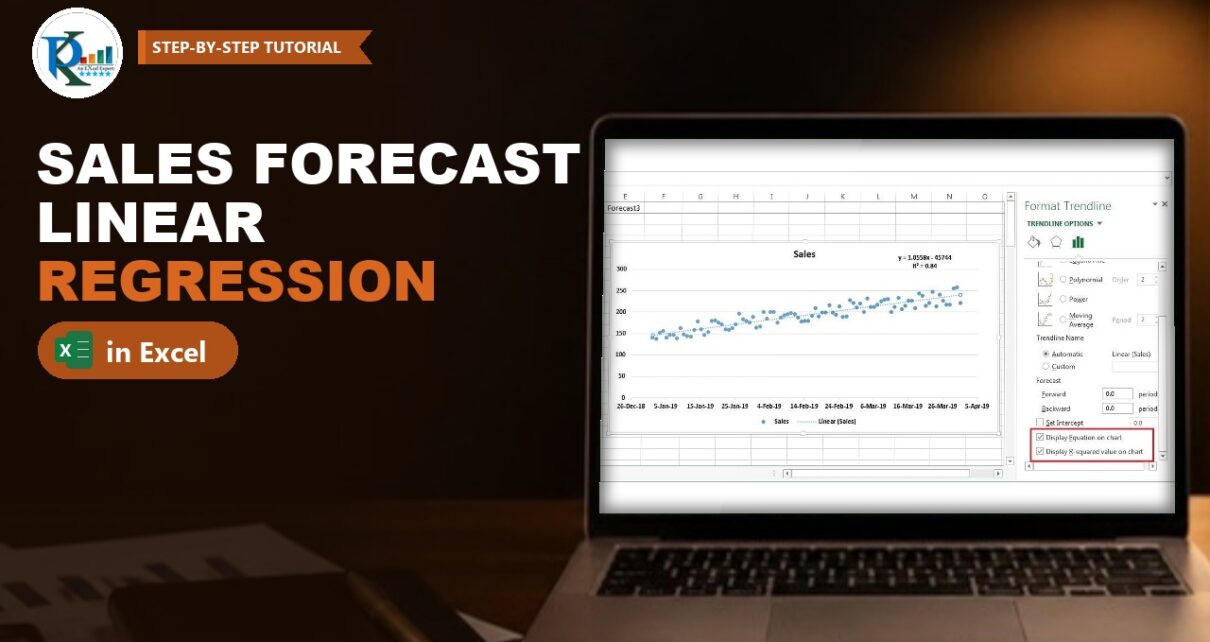
Click the chart, press the + (Chart Elements) button and tick Trendline → Linear. Excel fits a straight line through the dots using the least-squares method – that line is your linear regression. Right-click it and choose Format Trendline to change its colour or dash style.
Step 3: Show the equation and R-squared
In the Format Trendline pane keep Linear selected, scroll down and tick Display Equation on chart and Display R-squared value on chart. The chart now shows:
y = 1.0558x - 45744
R² = 0.84
Here y is sales and x is the date. The slope 1.0558 means sales grow by roughly one unit per day. An R-squared of 0.84 means the straight line explains about 84% of the day-to-day variation in sales, which is a good fit for daily data. In the practice file the trendline is also set to Forecast Forward 30 periods, so the dotted line continues through April.
Part 2 – Linear Regression Forecast Formulas in Excel
Method 1: The FORECAST function
FORECAST predicts a y-value for a new x-value along the least-squares line. The syntax is:
FORECAST(x, known_y's, known_x's)- x – the data point you want a prediction for (here, an April date).
- known_y’s – the dependent values you already have (the historical sales).
- known_x’s – the independent values that go with them (the historical dates).
In C92 enter the formula below, then fill it down to C121:
C92 =FORECAST(A92,$B$2:$B$91,$A$2:$A$91)Press F4 after selecting each historical range to lock it with $ signs. Only A92 stays relative, so each row picks up its own date. For 1-Apr-2019 the result is 241.37; for 30-Apr-2019 it is 271.99.
Method 2: The TREND function
TREND fits the same least-squares line and returns the values along it for the new x-values you give it:
TREND(known_y's, [known_x's], [new_x's], [const])
D92  =TREND($B$2:$B$91,$A$2:$A$91,A92)
Notice the order: known_y’s come first and the new date comes last, the opposite of FORECAST. The result is again 241.37. If you compare the two cells with an equals sign you may get FALSE, because of tiny differences far down in the decimal places, but the forecasts are the same for any practical purpose.
Method 3: The y = mx + c equation with SLOPE and INTERCEPT
A straight line is y = mx + c, where m is the slope and c is the intercept. Excel has a function for each, using the same known_y’s and known_x’s:
J1  =SLOPE($B$2:$B$91,$A$2:$A$91)        returns 1.055768
L1  =INTERCEPT($B$2:$B$91,$A$2:$A$91)    returns -45743.7
In the video these sit in helper cells J1 and L1, so the forecast is simply =$J$1*A92+$L$1. The practice file uses the all-in-one version, which needs no helper cells:
E92 =SLOPE($B$2:$B$91,$A$2:$A$91)*A92+INTERCEPT($B$2:$B$91,$A$2:$A$91)Fill it down to E121. Every row matches Methods 1 and 2. If the result looks like a date, change the cell format to Number or General.
Method 4: Use the chart equation directly
Copy the equation text from the chart label, paste it into F92 after an equals sign and replace x with the date cell:
F92 =1.0558*A92 - 45744This gives 242.42 for 1 April, about one unit higher than the other three. The reason is rounding: the chart label shows the slope as 1.0558 and the intercept as 45744, while the real values are 1.055768 and 45743.67. Multiplying a rounded slope by a date serial of about 43,556 magnifies the tiny rounding error.
How the formula works
- Excel stores dates as serial numbers. 1-Apr-2019 is 43556, so x is a large number and the regression line is calculated on those serials.
- The slope 1.0558 is the average increase in sales per day.
- The intercept -45743.7 is where the line would cross x = 0, which is a date in 1900. It has no business meaning on its own; it is just the constant that puts the line at the right height for 2019 dates.
- FORECAST, TREND and SLOPE × x + INTERCEPT all use the same least-squares line, which is why their results match.
Part 3 – Chart the Forecast
Select the dates, the Sales column and one forecast column and insert a line chart. Actual sales appear as one series up to 31 March and the forecast continues as a second, straight series through 30 April.
Modern Excel Alternatives (addition, not in the video)
The video uses the classic functions, which work in every version. Newer versions add these options:
- FORECAST.LINEAR (Excel 2016 and later) takes the same arguments as FORECAST and returns the same result. Microsoft keeps FORECAST for compatibility, so either name works:
=FORECAST.LINEAR(A92,$B$2:$B$91,$A$2:$A$91). - TREND as a spill formula (Microsoft 365 and Excel 2021): give TREND all the new dates at once and it fills all 30 rows from one cell:
=TREND(B2:B91,A2:A91,A92:A121). - RSQ returns the R-squared value in a cell instead of on the chart:
=RSQ(B2:B91,A2:A91)gives 0.84 for this data. - The FORECAST.ETS family (Excel 2016 and later) uses exponential triple smoothing (the AAA version of ETS) instead of a straight line, so it can follow seasonal patterns. FORECAST.ETS(target_date, values, timeline, [seasonality], [data_completion], [aggregation]) returns the prediction; FORECAST.ETS.CONFINT returns the confidence interval around it (95% by default); FORECAST.ETS.SEASONALITY returns the season length Excel detected; and FORECAST.ETS.STAT returns statistics about the model. The timeline needs a constant step, such as one row per day.
- Forecast Sheet (Data → Forecast → Forecast Sheet) builds an ETS forecast table and chart with upper and lower confidence bounds in a few clicks.
Use the linear methods in this tutorial when your data follows a steady straight-line trend, as it does here. Consider FORECAST.ETS when the data has a repeating seasonal pattern.
Common Errors and Fixes
The forecast shows a date instead of a number
The formula cell inherited a date format from the date column. Change it to Number or General.
Results drift as you fill down
The historical ranges were not locked. Use $B$2:$B$91 and $A$2:$A$91 so only the new date changes on each row.
#N/A or #VALUE! from FORECAST or TREND
The known_y’s and known_x’s ranges must be the same size and contain numbers. A text value or a blank date in the history, or ranges of different lengths, breaks the calculation.
The chart-equation forecast does not match the formulas
That is the rounding effect from Method 4. Right-click the equation label, choose Format Trendline Label and set a Number format with more decimal places, or simply use SLOPE and INTERCEPT.
Tips
- Always chart the history first. If the dots curve, jump around or repeat a seasonal pattern, a straight line will mislead you.
- Look at R-squared before trusting a linear forecast. The closer it is to 1, the better the straight line fits the history.
- Linear forecasts are most reliable for the near future. The further out you go, the more the real world can drift from the trend.
- Microsoft’s forecasting functions reference documents FORECAST.LINEAR and every FORECAST.ETS function.
Want It Ready-Made?
If you need a finished forecasting tool rather than building one, the Budget Forecasting Dashboard in Excel and the Forecast vs Actual Chart with Safe Zone Range on NextGenTemplates.com are ready to use, or you can browse all Excel analysis templates. To master FORECAST, TREND, SLOPE and the other formulas step by step, join the video course Excel + AI Mastery: 100 Essential Formulas and Real-World Projects.
Related Tutorials
- Correlation Coefficient in Excel
- Profit Optimizer in Excel using Multiple Regression
- Forecast vs Actual Chart with Safe Zone Range in Excel
- What-If Analysis in Excel: Goal Seek, Scenario Manager and Data Table
- Time Series Forecast and Anomaly Detection in Power BI
Frequently Asked Questions
How do I forecast sales in Excel using linear regression?
Put dates in one column and sales in the next, then use FORECAST with the new date as x, the historical sales as known_y’s and the historical dates as known_x’s. Lock the historical ranges with F4 and fill the formula down for every future date.
What is the difference between FORECAST and TREND in Excel?
Both fit the same least-squares straight line, so they return the same values. FORECAST takes the new x-value first, while TREND takes the known values first and the new x-values last. TREND can also return many results at once.
Is FORECAST.LINEAR different from FORECAST?
No. FORECAST.LINEAR was added in Excel 2016 with the same arguments and the same result. FORECAST is kept for compatibility with older workbooks.
What does an R-squared value of 0.84 mean?
It means the straight trendline explains about 84 percent of the variation in the historical sales. Values closer to 1 indicate a tighter fit, so a linear forecast is more trustworthy.
Why does the chart equation give a slightly different forecast?
The trendline label rounds the slope and intercept. Because Excel dates are large serial numbers, even a small rounding in the slope shifts the result by about one unit here. SLOPE and INTERCEPT use full precision.
When should I use FORECAST.ETS instead of a linear forecast?
Use FORECAST.ETS when your history has a repeating seasonal pattern, such as weekly or yearly peaks. A linear forecast suits data that rises or falls along a steady straight-line trend, like the sales in this tutorial.
About the Author
PK is a Microsoft Excel expert and trainer and the founder of PK: An Excel Expert and NextGenTemplates.com. He has been teaching Excel, Power Query and Power BI since 2016 on his YouTube channel.
Conclusion
Forecasting in Excel using linear regression comes down to one straight line fitted through your history. Chart the data and check the R-squared, then let FORECAST, TREND or SLOPE and INTERCEPT extend that line into the future: all three return the same numbers, while the chart equation is a handy shortcut once you allow for rounding. Download the practice file, change the sales and watch the April forecast update instantly.