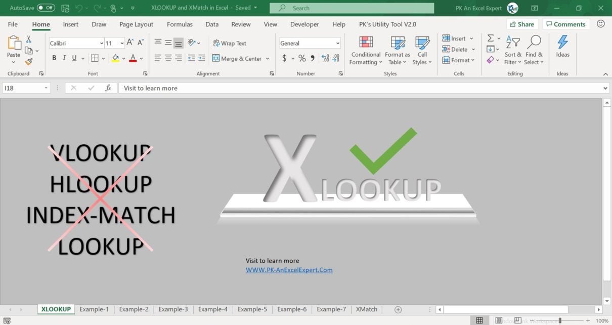
In this article, You will learn how to use XLOOKUP and XMATCH Function in Microsoft Excel. XLOOKUP is very powerful functions. This function is currently available to Microsoft 365 subscribers in Current Channel of Office Insider. XLOOKUP can be used in place of VLOOKUP, HLOOKUP, INDEX–MATCH etc. XLOOKUP supports approximate and exact matching, wildcards (* ?) for partial matches. It can lookup in vertical and horizontal both type of ranges.
XLOOKUP and XMATCH Function in Excel
Below the example and explanation of XLOOKUP and XMATCH Function
XLOOKUP
Syntax
=XLOOKUP (lookup_value, lookup_array, return_array, [if_not_found], [match_mode], [search_mode])
Arguments
- lookup_value – The lookup value.
- lookup_array – The array or range to search.
- return_array – The array or range to return.
- If_not_found – [optional] Value to return if no match found.
- match_mode – [optional] 0 = exact match (default), -1 = exact match or next smallest, 1 = exact match or next larger, 2 = wildcard match.
- search_mode – [optional] 1 = search from first (default), -1 = search from last, 2 = binary search ascending, -2 = binary search descending.
Watch the step by step video tutorial for XLOOKUP and XMATCH Function:
Below are the few examples of XLOOKUP
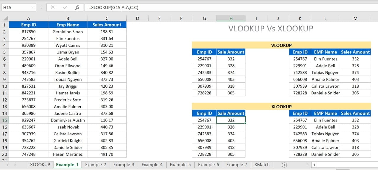
Example #1: XLOOKUP in place of VLOOKUP
We can use XLOOKUP in place of VLOOKUP. As given in below image to get the Sale Amount on the base of EMP Id, we can use
=XLOOKUP(G15,A:A,C:C)
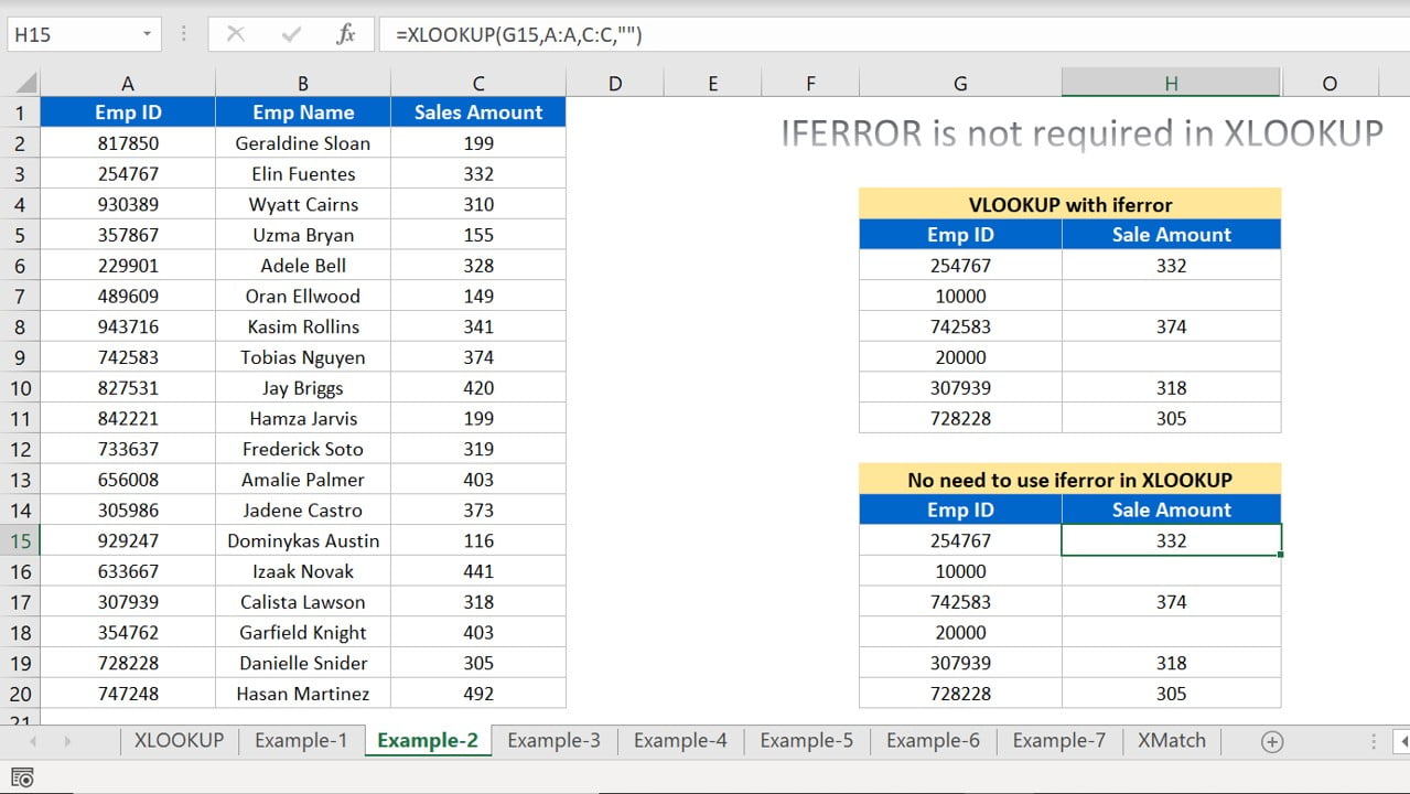
Example #2: No need to use IFERROR in XLOOKUP
We use IFERROR with VLOOKUP to handle the potential error, which may occur if lookup value not found in lookup array. XLOOKUP has an additional argument “[If_not_found]” in its syntax. You can use some text here so it will return that text in place of error.
=XLOOKUP(G15,A:A,C:C,"")
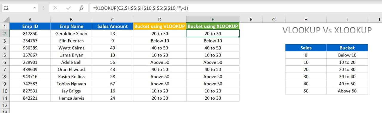
Example #3: Approximate match with XLOOKUP
XLOOKUP provides the 4 type of match mode – exact match (default), -1 = exact match or next smallest, 1 = exact match or next larger, 2 = wildcard match. In the blow example, we have used to create the sales bucket
=XLOOKUP(C2,$H$5:$H$10,$I$5:$I$10,"",-1)
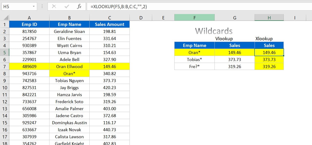
Example #4: Wildcard with XLOOKUP
In the match mode, 4th option is for Wildcard. In the below given image we have used wildcard in XLOOKUP to get the sales by partial employee name-
Learn how to use Wildcard in Microsoft Excel
=XLOOKUP(F5,B:B,C:C,"",2)
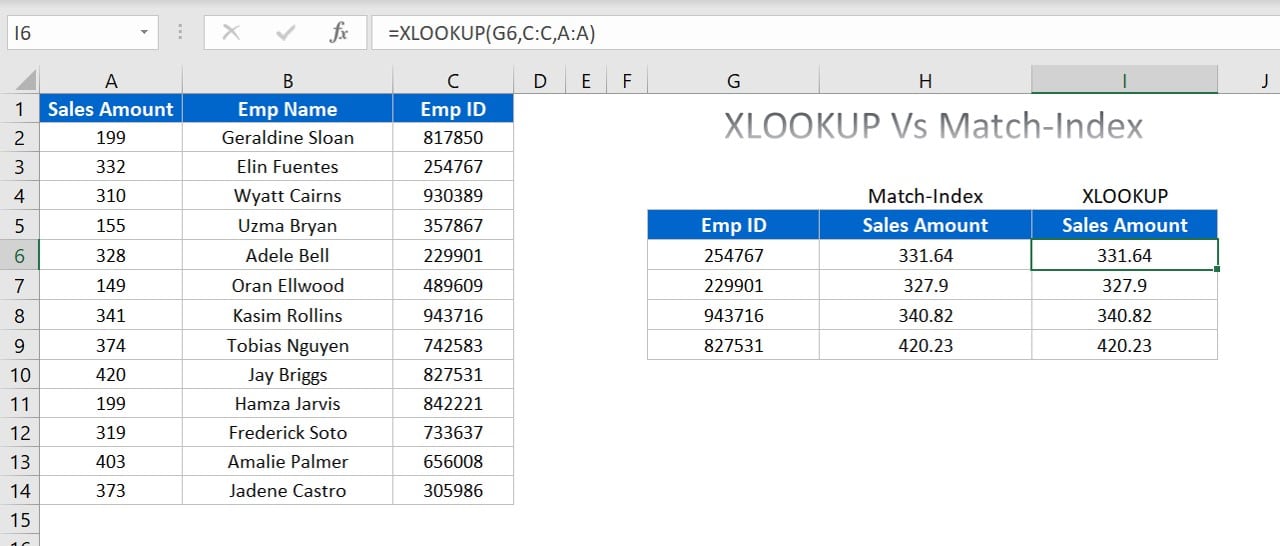
Example #5 XLOOKUP in place of INDEX – MATCH
Unlike VLOOKUP, we have used XLOOKUP form Right to Left. So we don’t need to use INDEX and MATCH function. In the below image we have used XLOOKUP to get the Sales amount on the base of EMP ID
=XLOOKUP(G6,C:C,A:A)
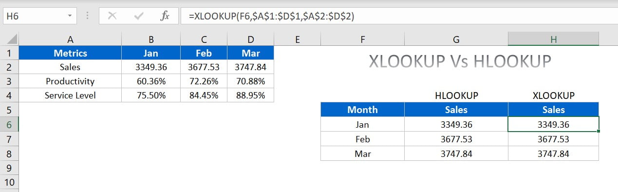
Example #6 XLOOKUP in place of HLOOKUP
XLOOUP works in both direction – Vertically and Horizontally. So in place of HLOOKUP we can use XLOOKUP. In the below given image, we have used XLOOKUP to get the Sales for Months
=XLOOKUP(F6,$A$1:$D$1,$A$2:$D$2)
Learn how to use HLOOKUP in Excel:
Example #7 Search from Last to First
In the XLOOKUP, we can search from last to first also. If you have duplicate values in your lookup arrays, then you can get the result for last occurrence also. In the below image we have used search mode as -1, which is for “search last to first”
=XLOOKUP(I6,C:C,D:D,"",0,-1)

XMATCH
XMATCH is same as MATCH function but it is more powerful than Match function. supports approximate and exact matching, wildcards (* ?) for partial matches. It can lookup in vertical and horizontal both type of ranges.
Syntax
=XMATCH (lookup_value, lookup_array, [match_mode], [search_mode])
Example:
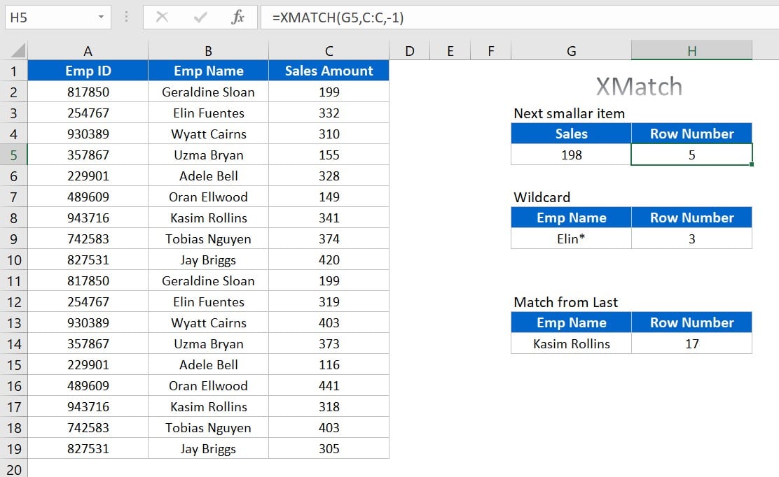
In the below image, we have used XMATCH to get the row number, wherein Sales Amount is exact 198 or next smaller of 198.
=XMATCH(G5,C:C,-1)
We can use the wildcards with XMATCH. To get the row number for an employee on the base of Partial name we can use-
=XMATCH(G9,B:B,2)
We can match for the last also. We have duplicate values in lookup array, we can use search mode as last to first
=XMATCH(G14,B:B,0,-1)