Part of the free Module 5: Excel Formulas and Functions · Function 56 of 105 · Full Excel course
Updated on 5 September 2026 · Works in Excel 365, 2021, 2019 and 2016 (and earlier).
The Excel MATCH function searches one row or one column for a value and returns its relative position as a number, not the value itself. MATCH in Excel answers the question “which row is this item in?”, which makes it the natural partner for INDEX, a quick way to test whether a value exists in a list, and the engine behind two-way lookups.
MATCH syntax
=MATCH(lookup_value, lookup_array, [match_type])| Argument | Required or optional | What it does | Notes and defaults |
|---|---|---|---|
lookup_value |
Required | The value to find: a number, text, logical value or a cell reference to one of these. | Text comparison is not case-sensitive. With match_type 0 you can use the wildcards ? (one character) and * (any characters). |
lookup_array |
Required | The range or array to search. It must be a single row or a single column. | A two-dimensional range returns #N/A. |
match_type |
Optional | Controls how MATCH compares values. | 0: exact match, any order, first hit wins. 1 or omitted: largest value less than or equal to lookup_value; lookup_array must be sorted ascending. -1: smallest value greater than or equal to lookup_value; lookup_array must be sorted descending. |
The three match_type values in detail:
| match_type | Meaning | Sort order required | Typical use |
|---|---|---|---|
| 0 | Exact match. Returns the position of the first cell equal to lookup_value. | None | IDs, names, codes; almost every lookup |
| 1 (default) | Approximate. Returns the position of the largest value that is less than or equal to lookup_value. | Ascending | Tax slabs, grade bands, commission tiers |
| -1 | Approximate. Returns the position of the smallest value that is greater than or equal to lookup_value. | Descending | Thresholds listed high to low, such as discount cut-offs |
How MATCH works
MATCH returns a whole number between 1 and the size of lookup_array. The number is relative to the range, not to the worksheet: =MATCH("Delhi", A5:A20, 0) returning 1 means Delhi is in A5. If no cell qualifies, MATCH returns #N/A. With match_type 0 Excel scans from the top and stops at the first equal value, so duplicates always return the first occurrence. With match_type 1 or -1 Excel uses a binary search, which is faster on long lists but assumes the data is sorted; on unsorted data it returns plausible but wrong positions.
Version notes. MATCH behaves the same in every version of Excel and in Google Sheets. Excel 365 and Excel 2021 add XLOOKUP, which combines INDEX and MATCH into one function with an exact match by default, and XMATCH, which is MATCH with exact match as the default and a search-from-last option. Use MATCH when a workbook must open in Excel 2019 or earlier, or when you need a position rather than a value.
Worked examples
Example 1: Find the position of a value in a list
City names are in A2:A6. You want to know where Delhi sits.
| A (City) | Formula | Result |
|---|---|---|
| Mumbai | =MATCH("Delhi", A2:A6, 0) |
4 |
| Chennai | ||
| Kolkata | ||
| Delhi | ||
| Pune |
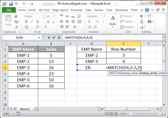
Delhi is the fourth cell of A2:A6, so MATCH returns 4 even though Delhi is in sheet row 5. The screenshot below shows the same idea on a longer list.
Example 2: INDEX and MATCH lookup that works in any direction
Employee IDs are in column A, names in B and salaries in C. A lookup ID is typed in F2. This is the classic replacement for VLOOKUP because it can return from any column, including ones to the left of the lookup column, and it does not break when columns are inserted.
| A (ID) | B (Name) | C (Salary) | F2 (Lookup ID) | Formula | Result |
|---|---|---|---|---|---|
| E101 | Asha | 52,000 | E103 | =INDEX($C$2:$C$5, MATCH(F2, $A$2:$A$5, 0)) |
61,500 |
| E102 | Rahul | 48,000 | |||
| E103 | Meera | 61,500 | |||
| E104 | Vikram | 45,000 |
MATCH finds E103 in the third position of A2:A5; INDEX returns the third value of C2:C5. To return the name instead, point INDEX at B2:B5 and leave MATCH unchanged.
Example 3: Two-way lookup with INDEX and two MATCH functions
A sales grid has regions down column A and months across row 1. Region is in G1 and month in G2.
| B (Jan) | C (Feb) | D (Mar) | |
|---|---|---|---|
| North | 120 | 135 | 150 |
| South | 98 | 110 | 125 |
| East | 76 | 82 | 90 |
=INDEX($B$2:$D$4, MATCH(G1, $A$2:$A$4, 0), MATCH(G2, $B$1:$D$1, 0))With G1 = South and G2 = Feb, the row MATCH returns 2, the column MATCH returns 2, and INDEX returns 110. Swapping either input re-points the formula instantly.
Example 4: Dynamic column number inside VLOOKUP
Hard-coded column numbers break when someone inserts a column. Let MATCH find the column by its header instead.
=VLOOKUP(A2, $H$1:$M$500, MATCH("Amount", $H$1:$M$1, 0), FALSE)MATCH returns the position of the Amount header within H1:M1, and VLOOKUP uses that as col_index_num. Rename or move the column and the formula still finds it.
Example 5: Test whether a value exists, and wildcard matching
| Goal | Formula | Result |
|---|---|---|
| Is the value in A2 present in D2:D100? | =IF(ISNUMBER(MATCH(A2, $D$2:$D$100, 0)), "Yes", "No") |
Yes or No |
| Position of the first company ending in Ltd | =MATCH("*Ltd", A2:A100, 0) |
Position of the first match |
| Position of a five-character code starting with AB | =MATCH("AB???", A2:A100, 0) |
Position of the first match |
| Grade band for a score of 83 (thresholds 0, 50, 70, 90 in D2:D5) | =INDEX(E2:E5, MATCH(83, D2:D5, 1)) |
Grade in E4 |
ISNUMBER turns the position into TRUE and the #N/A into FALSE, which is the standard way to check membership without an error. Wildcards work only with match_type 0.
Tips and common mistakes
- Always type the 0. Omitting match_type means approximate match on ascending data, which returns wrong positions on an unsorted list without any warning.
- Anchor the ranges. Use $A$2:$A$500 before copying INDEX and MATCH down, and make sure INDEX and MATCH cover the same rows.
- Clean the data first. A trailing space or a number stored as text is the usual reason MATCH says #N/A for a value you can see. Wrap in TRIM or VALUE.
- Position is not the row number. Add the offset (start row minus 1) if you need the sheet row, or use ROW() arithmetic. Better still, pass the same range to INDEX.
- Duplicates return the first hit. For the last occurrence use XMATCH with search_mode -1 in Excel 365, or the LOOKUP(2, 1/(range=value), …) pattern in older versions.
- Use a Table. Structured references such as Sales[ID] grow automatically, so MATCH never misses new rows.
- Move to XLOOKUP when you can. In Excel 365 and 2021 one XLOOKUP replaces INDEX and MATCH, matches exactly by default and has a built-in if_not_found argument.
Errors and how to fix them
| Error | Cause | Fix |
|---|---|---|
| #N/A | No match found: the value is absent, differs by a space or data type, lookup_array is two-dimensional, or match_type 1 or -1 was used on unsorted data. | Use TRIM and VALUE, set match_type to 0, select a single row or column, or wrap in IFNA for a friendly message. |
| #VALUE! | match_type is text or lookup_array is not a valid range or array. | Use 0, 1 or -1 and a proper range reference. |
| #REF! | lookup_array points at cells that were deleted. | Re-select the range. |
| #NAME? | The function or a named range is misspelt, for example MACH. | Correct the spelling. |
| Wrong position, no error | match_type omitted on unsorted data, or INDEX and MATCH cover different ranges. | Type 0 as the third argument and align the ranges. |
Practice exercise
- Type the five cities from Example 1 into A2:A6 and find the position of Kolkata. Expected: 3.
- Build the employee table from Example 2 and return the name for ID E104 using INDEX and MATCH. Expected: Vikram.
- Create the region and month grid from Example 3 and return the March figure for East. Expected: 90.
- Add a column of Yes or No that shows whether each ID in a second list exists in the employee table. Expected: Yes for E101 to E104, No for anything else.
- Delete the third argument from one MATCH formula, shuffle the list and observe the result. Expected: a wrong position, which shows why match_type 0 matters.
Key takeaways
- MATCH returns a position number, not a value; INDEX turns that position into a value.
- Use match_type 0 for almost everything; 1 and -1 are for sorted banded data.
- INDEX and MATCH look up in any direction and survive inserted columns, unlike VLOOKUP.
- Two MATCH functions inside INDEX give a two-way lookup by row and column header.
- ISNUMBER(MATCH(…)) is the standard test for whether a value exists in a list.
- In Excel 365 and 2021, XLOOKUP and XMATCH do the same jobs with fewer arguments.
Related functions and lessons
- Excel Formulas and Functions library: every function page in this module.
- INDEX: returns the value at the position MATCH finds.
- VLOOKUP and HLOOKUP: classic table lookups that MATCH can make more robust.
- XLOOKUP and XMATCH step-by-step tutorial: the modern one-function replacement for INDEX and MATCH in Excel 365 and 2021.
- LOOKUP: the older approximate-match function.
- ISNA and ISNUMBER: test the result of MATCH.
- Two-way lookup using INDEX, MATCH and MATCH.
- INDEX MATCH vs VLOOKUP vs XLOOKUP compared.
- Excel Dashboard course: INDEX and MATCH drive most interactive dashboard selectors.
- Microsoft Support: MATCH function.
Frequently asked questions
What does the MATCH function return in Excel?
MATCH returns a number that shows the relative position of the lookup value inside the range you searched. If the range starts at A5 and the value is in A7, MATCH returns 3, not 7. The number is meant to be fed to INDEX, CHOOSE or OFFSET, which then return the actual value from that position.
Why does MATCH give #N/A when the value is in the list?
Excel does not see the two values as identical. The usual causes are a trailing or leading space, a number stored as text on one side and a real number on the other, or a missing match_type so Excel performed an approximate match on unsorted data. Clean with TRIM or VALUE and type 0 as the third argument.
What is the difference between MATCH and XMATCH?
XMATCH, available in Excel 365 and 2021, defaults to exact match instead of approximate, adds a search_mode argument that can search from the last item or use a binary search, and supports a wildcard match mode explicitly. MATCH remains the choice for workbooks that must open in Excel 2019 or earlier.
Can MATCH search a two-dimensional range?
No. lookup_array must be a single row or a single column, otherwise MATCH returns #N/A. To search a grid, use INDEX with two MATCH functions, one to find the row from the first column and one to find the column from the header row, as shown in Example 3.
Is INDEX MATCH better than VLOOKUP?
For most professional workbooks, yes. INDEX and MATCH can return a column to the left of the lookup column, keep working when columns are inserted or deleted, and only read the two columns involved rather than the whole table, which is faster on large data. VLOOKUP is shorter to type and fine for simple, stable tables.
Want the finished version? Ready-made Excel dashboards, trackers and VBA systems built with these functions are available at NextGenTemplates.com.