Excel VLOOKUP Function: Syntax, Examples and Errors

Part of the free Module 5: Excel Formulas and Functions · Function 97 of 105 · Full Excel course

The Excel VLOOKUP function searches for a value in the first column of a table and returns a value from another column in the same row. Use VLOOKUP in Excel when you need to pull a price, name, rate or status from a reference table into your working sheet. It returns the matched value, or #N/A when nothing matches.

Table of Contents

VLOOKUP syntax

=VLOOKUP(lookup_value, table_array, col_index_num, [range_lookup])

Arguments

Argument	Required	Meaning
lookup_value	Required	The value to search for. It must appear in the first column of table_array. Can be a number, text or a cell reference.
table_array	Required	The range that holds the data. The lookup column must be the left-most column of this range.
col_index_num	Required	The column number inside table_array to return from. 1 is the lookup column, 2 is the next column to the right, and so on.
range_lookup	Optional	FALSE (or 0) for an exact match. TRUE, 1 or omitted for an approximate match, which requires the first column to be sorted ascending.

Step-by-step example

Suppose column A holds an Employee ID you type in, and the master table sits in B2:D8 with ID, Name and Department. To return the name for the ID in A2:

=VLOOKUP(A2, B2:D8, 2, FALSE)

Excel reads the value in A2.
It scans the first column of B2:D8 (column B) from top to bottom for an exact match.
When it finds the row, it moves to column 2 of the range (column C) and returns that cell.
If no row matches, the formula returns #N/A.

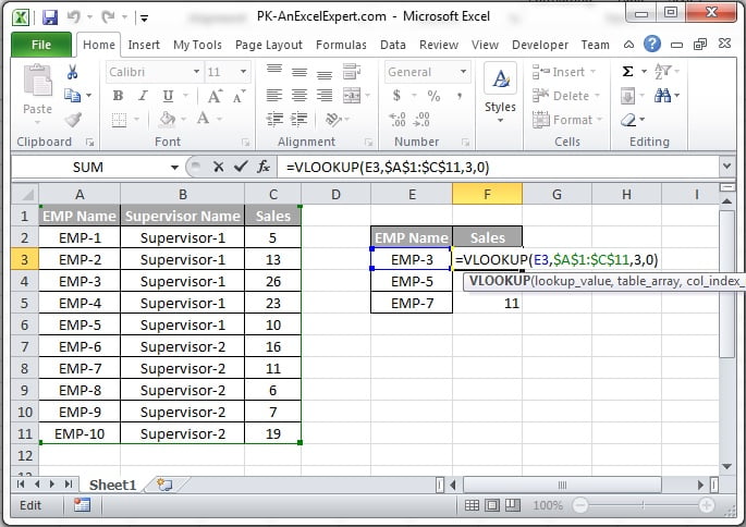
The screenshot below shows the same idea on a product list: the product code is entered once and VLOOKUP fills in the matching details from the table.

Excel VLOOKUP function example showing an exact-match lookup that returns a value from a product table — VLOOKUP Formula Example

Exact match vs approximate match

Exact match (FALSE)

Use FALSE for IDs, codes, names and anything where a near miss is wrong. The data does not need to be sorted. This is the setting you want in more than 90% of real cases.

Approximate match (TRUE)

Use TRUE for banded lookups such as tax brackets, commission tiers or grade boundaries. VLOOKUP returns the largest value that is less than or equal to lookup_value, so the first column must be sorted in ascending order. For example, with score bands 0, 50, 70, 90 in E2:E5 and grades in F2:F5:

=VLOOKUP(B2, E2:F5, 2, TRUE)

Practical use cases

1. Lock the table with absolute references

When you copy the formula down, keep the table fixed so it does not shift:

=VLOOKUP(A2, $H$2:$K$500, 3, FALSE)

2. Handle missing values with IFERROR

=IFERROR(VLOOKUP(A2, $H$2:$K$500, 3, FALSE), "Not found")

3. Pull data from another sheet

=VLOOKUP(A2, Prices!$A$2:$C$300, 3, FALSE)

4. Look left with INDEX and MATCH

VLOOKUP can only return columns to the right of the lookup column. When the value you need sits to the left, or you want the formula to survive inserted columns, use INDEX-MATCH:

=INDEX($B$2:$B$500, MATCH(A2, $D$2:$D$500, 0))

XLOOKUP note: In Excel 365 and Excel 2021, =XLOOKUP(A2, D2:D500, B2:B500, "Not found") does the same job with no column number, looks in any direction and defaults to exact match. Keep VLOOKUP for files shared with older Excel versions.

Common mistakes and errors

#N/A – the value is not in the first column. Check for extra spaces (wrap with TRIM), numbers stored as text, or an omitted FALSE that triggered an approximate match on unsorted data.
#REF! – col_index_num is larger than the number of columns in table_array. Count the columns in the range, not in the sheet.
#VALUE! – col_index_num is 0, negative or text. It must be a positive whole number.
Wrong result after inserting a column – the hard-coded column number no longer points at the right field. Use INDEX-MATCH or MATCH("Header", H1:K1, 0) to compute the column dynamically.
Only the first match is returned – VLOOKUP stops at the first hit. For multiple matches use FILTER (Excel 365) or a helper column.

Related functions

HLOOKUP – the horizontal version, searching the first row instead of the first column.
INDEX and MATCH – the flexible pair that replaces VLOOKUP in complex models.
IFERROR – wraps VLOOKUP to replace #N/A with a friendly message.
XLOOKUP and XMATCH tutorial and VLOOKUP by cell background colour.
Browse every lesson in the Excel Formulas hub.

Frequently asked questions

Why does VLOOKUP return #N/A even though the value exists?

Usually the two cells are not identical: one has a trailing space or is a number stored as text. Wrap the lookup value in TRIM or VALUE, or use Text to Columns to convert the table column to real numbers.