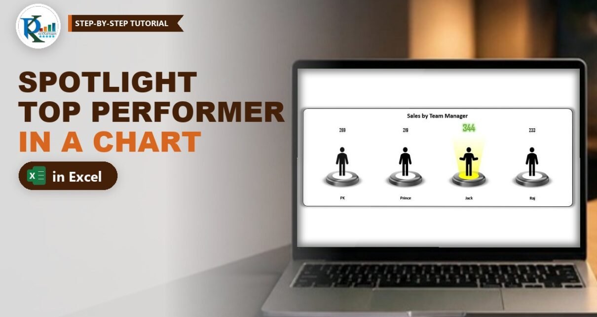
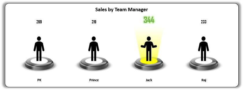
Want to highlight the top performer in an Excel chart so nobody has to hunt for the biggest number? In this second part of the spotlight visualization series you build a column chart of sales by team manager where the person with the highest sales stands under a glowing yellow spotlight, and everyone else stands on an unlit stage. Four small helper formulas decide who gets the light, so the spotlight moves on its own when the numbers change. You also build an optional 3-D floor to place the chart on.
Watch the Video Tutorial
PK reuses the spotlight from Part 1, adds four helper columns, pastes the lit and unlit spotlights into a clustered column chart, and finishes with a perspective floor made from 60 rectangles.
What You Will Build
- Four helper columns that flag the highest sale with MAX and hide the other values with NA().
- A lit and an unlit stage built from the Part 1 spotlight, each with a person icon.
- A clustered column chart whose columns are filled with those pictures instead of colour.
- Smart data labels: plain black numbers for everyone, a large glowing green number for the winner.
- Variant 2: the same chart standing on a textured 3-D floor.
Step 1 – The Data and the Helper Columns
The source data is just two columns: the team managers PK, Prince, Jack and Raj, and their sales. In the video it sits in A1:B5 (headers in row 1). While building, PK uses RANDBETWEEN for the sales so that pressing F9 gives new numbers and you can test that the spotlight moves.
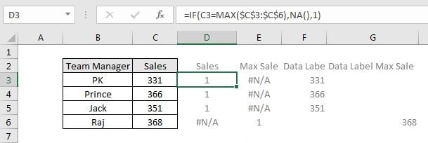
Add four helper headers in C1:F1: Sales, Max Sale, Sales Data Label and Max Sale Data Label. Then enter these formulas in row 2 and fill them down to row 5:
C2  =IF(B2=MAX($B$2:$B$5),NA(),1)
D2  =IF(B2=MAX($B$2:$B$5),1,NA())
E2  =IF(B2=MAX($B$2:$B$5),"",B2)
F2  =IF(B2=MAX($B$2:$B$5),B2,"")
Press F4 after selecting the range inside MAX so it stays locked as you fill down.
How the formulas work
B2=MAX($B$2:$B$5)is TRUE only on the row with the highest sale.- Sales (C) returns 1 for every manager except the winner, who gets
#N/A. This series will carry the unlit stage. - Max Sale (D) is the mirror image: 1 for the winner and
#N/Afor everyone else. This series carries the lit spotlight. - Because every visible column has the same height of 1, all the stages are the same size. The real sales numbers are shown through labels instead.
- Charts skip
#N/Avalues, so on each row only one of the two columns is drawn. That is what makes the light jump from person to person. - Sales Data Label (E) shows the sale for everyone except the winner; Max Sale Data Label (F) shows only the winner’s sale.
Step 2 – Prepare the Lit and Unlit Spotlights
Start with the yellow spotlight you built in Part 1 of this spotlight series and make a copy of it.
- Lit stage – keep the first copy exactly as it is: yellow disc, yellow beam.
- Unlit stage – in the second copy, set the beam’s transparency to 100% so the light disappears, and fill the small inner oval with white.
PK then places a person icon on each stage: one standing with arms down for the unlit stage and one with open arms for the lit stage. Select each icon with its stage and Group them. Finally select the big outer oval, open Format Shape → Effects → 3-D Format and reduce the bevel Depth from 25 pt to 10 pt so the stages look slimmer inside the chart. Turn off gridlines in View as well.
Step 3 – Highlight the Top Performer in the Excel Chart
Insert the column chart
Select the Team Manager column together with the two helper series, Sales and Max Sale (hold Ctrl to select non-adjacent columns). Go to Insert → Charts → Clustered Column.
Fix the axis
Right-click the vertical axis and choose Format Axis. Set Minimum to 0 and Maximum to 1.1, which leaves a little headroom above the columns for the labels. Then delete the vertical axis and the legend; they are not needed.
Paste the pictures into the columns
This is the clever part. Select and copy the lit spotlight group, click the Max Sale series in the chart and press Ctrl+V. The column is now filled with the spotlight picture. Copy the unlit group, click the Sales series and paste again. Every column now shows a stage.
Line the stages up
Right-click a series, choose Format Data Series and set Series Overlap to 100% and Gap Width to 0%. With full overlap, the lit and unlit columns share the same slot, so the winner’s stage sits exactly where an unlit stage would have been. Remove the gridlines from Chart Elements. You can give the chart a white background, a border and a soft shadow if you like.
Step 4 – Add Labels from Cells
Labels for everyone else
Right-click the Sales series and choose Add Data Labels, then Format Data Labels. Tick Value From Cells and select the Sales Data Label range (E2:E5) – make sure all four rows are selected. Untick Value and Show Leader Lines. Format the labels black, bold, a little bigger, in the Agency FB font.
The winner’s label
Do the same for the Max Sale series, but point Value From Cells at the Max Sale Data Label range (F2:F5). Make this label green, bold and larger (around 18 to 20 pt) in Agency FB, then go to Format → Text Effects → Glow to make the number shine like it does in the screenshot.
Add a chart title such as Sales by Team Manager. Now press F9: the sales change, the helper formulas move the 1 and the #N/A, and the spotlight and the green number jump to the new leader.
Step 5 – Variant 2: Put the Chart on a 3-D Floor
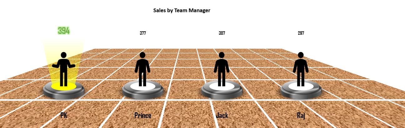
Build the tiles
Add a new sheet and switch off its gridlines. Insert one rectangle, then press Ctrl+D until you have 10. Select them all, copy and paste until you have 60 rectangles of the same size.
Arrange them in a grid
The rectangles need to sit in 6 rows of 10 with an equal gap. PK does this in one click with the free PK’s Utility Tool add-in: Object Manager → Horizontal grid, spacing 3 pt, 6 rows. Without the add-in you can line them up with Align Left/Top and Distribute Horizontally/Vertically. Then right-click and Group the 60 tiles.
Tilt the floor
Open Format Shape → Effects → 3-D Rotation, choose the Perspective Relaxed preset and adjust it to X rotation 0°, Y rotation about 300° (299.6° in the video) and Perspective 120°. Under 3-D Format set the Material to Metal and keep the default lighting. Finally use Fill → Picture or texture fill and pick a texture you like.
Place the chart
Copy the chart from the first sheet and paste it on the floor. Set the chart area and plot area to No fill and No outline, remove the shadow, and make the horizontal axis labels black, around 15 pt, Agency FB so the names stay readable on the texture.
Modern Excel Alternative
This section is an addition and is not shown in the video. In Microsoft 365 you can find people icons under Insert → Icons instead of downloading pictures, and recolour them with Graphics Fill. If you prefer one formula per helper, LET keeps the MAX in one place:
=LET(top,MAX($B$2:$B$5),IF(B2=top,1,NA()))It works exactly like the Max Sale formula above, but the range is only typed once.
Common Errors and Fixes
Two stages appear side by side for the winner
Series Overlap is not 100%. Set it to 100% and Gap Width to 0% in Format Data Series.
Two people get the spotlight
That happens when two managers tie for the highest sale, because both rows match MAX. If you want only the first top seller to get the light, compare the row position with MATCH instead, for example in the Max Sale helper:
=IF(ROWS($B$2:B2)=MATCH(MAX($B$2:$B$5),$B$2:$B$5,0),1,NA())Use the same test in the other three helpers.
The stages look squashed or stretched
A pasted picture stretches to fill the column. Keep the axis maximum at 1.1 and resize the chart until the stages look round again.
Tips
- Swap MAX for MIN in the four formulas to spotlight the lowest performer instead.
- Replace RANDBETWEEN with your real data, or link the sales to a pivot table summary.
- Keep both spotlight groups on a hidden sheet so you can re-paste them if you change the design.
- Microsoft’s page on the NA function explains why #N/A values are skipped in charts.
Want It Ready-Made?
If you want the finished workbook with both variants, get Spotlight Visualization in Excel (Part-2) from NextGenTemplates.com, or explore more Excel charts and visualization templates. To go deeper into charts, infographics and dashboards, take the course Excel Pivot Tables and Dashboards.
Related Tutorials
- Spotlight Visualization in Excel (Part 1): Dynamic RAG Stoplights
- Highlight Top and Bottom Performers with Conditional Formatting
- Highlight a Specific Data Point in a Line Chart Dynamically
- Column Chart in Excel: Clustered Column Step by Step
- Top and Bottom Sales Analysis Dashboard in Excel
Frequently Asked Questions
How do I highlight the highest value in an Excel chart automatically?
Split the data into two helper series with IF and MAX: one that holds only the highest value and one that holds all the others, using NA() for the missing points. Format the two series differently and set Series Overlap to 100%.
Why use NA() instead of a blank in the helper columns?
Excel charts skip #N/A values completely, so the hidden column does not take up space or show as zero. A blank text result or a zero can still be plotted.
How do I put a picture inside a chart column?
Copy the shape or picture, click the data series in the chart and press Ctrl+V. The picture fills every column of that series.
Can I spotlight the lowest performer instead?
Yes. Replace MAX with MIN in the four helper formulas and the spotlight moves to the lowest value.
Do I need the PK Utility Tool for the floor?
No. It only speeds up arranging the 60 rectangles into a grid. You can do the same with the Align and Distribute commands on the Shape Format tab.
About the Author
PK is a Microsoft Excel expert and trainer and the founder of PK: An Excel Expert and NextGenTemplates.com. He has been teaching Excel, Power Query and Power BI since 2016 on his YouTube channel.
Conclusion
To highlight the top performer in an Excel chart, you only need two helper series driven by IF, MAX and NA(), plus two label columns. Fill the columns with a lit and an unlit spotlight, overlap them 100%, and the light follows the leader every time the data changes. Add the perspective floor for a presentation-ready infographic, and pair it with the RAG lights from Part 1 for a complete spotlight dashboard.