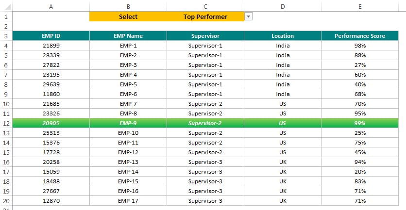
In this article you will learn how to use Conditional Formatting to Highlight Top and Bottom performer on the base of performance score. Top performer has been highlighted in green color and Bottom performer has been highlighted in red color. A drop-down of Top Performer and Bottom performer has been given on cell C1 using Data Validation list.
In the below image, top performer has been highlighted. To highlight the top performer we have the put the below formula in Conditional formatting:
“=AND($C$1=”Top Performer”,$E4=MAX($E$4:$E$20))“
Highlight Top and Bottom
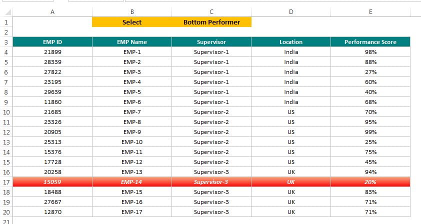
In the below image, bottom performer has been highlighted. To highlight the bottom performer we have the put the below formula in Conditional formatting:
“=AND($C$1=”Bottom Performer”,$E4=MIN($E$4:$E$20))“
Click here to download this Excel file.
Watch the step by step video tutorial to learn:
Visit our YouTube channel to learn step-by-step video tutorials