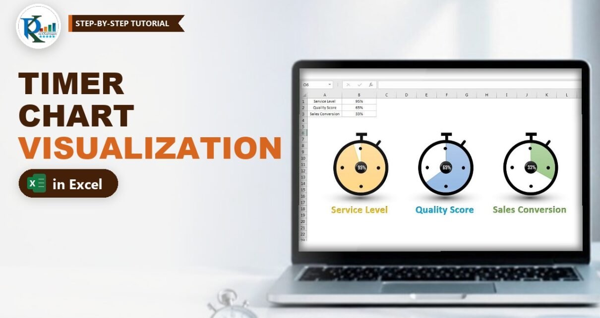
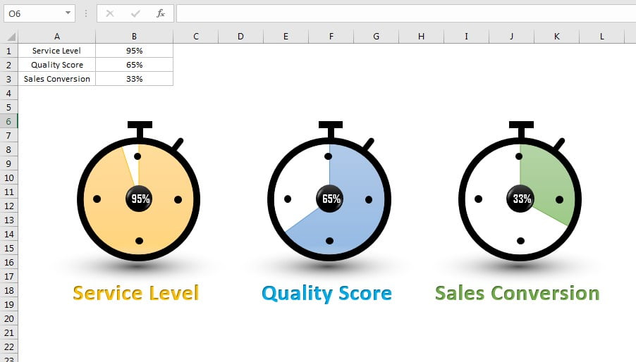
A timer chart visualization in Excel turns a plain percentage into a stopwatch whose face fills up as the value grows. It is a great way to show KPI metrics such as Service Level, Quality Score or Sales Conversion on a dashboard or in a presentation. In this tutorial you build it from a 2-D pie chart and a handful of Excel shapes: a donut ring, small dots, a rectangle crown and a soft shadow. The chart is fully data driven, so when you type a new value in the cell, the filled area and the label in the centre update instantly.
Watch the Video Tutorial
In the video PK draws the stopwatch from shapes, places a borderless pie chart behind it, links a WordArt label to the value cell and then copies the finished timer for the other two KPIs.
What You Will Build
- A stopwatch shape made from a donut, four dots, a crown and a side button, grouped into one object.
- A 2-D pie chart behind the ring that fills clockwise from 12 o’clock as the percentage grows.
- A live value label in the centre, linked to the KPI cell.
- A soft floor shadow made with a path gradient.
- Three colour-coded KPI timers (orange, blue and green) aligned in one row.
Part 1 – Prepare the Data
Step 1: Enter the KPIs
Type the metric names in A1:A3 (Service Level, Quality Score, Sales Conversion) and their values as percentages in B1:B3.
Step 2: Add the support column
A pie chart needs two slices: the value and the rest of the circle. In C1 enter the formula below and fill it down to C3:
C1 =1-B1With 95% in B1, C1 returns 5%. This second slice becomes the transparent part of the timer face, so B plus C always adds up to 100% and the pie always forms a full circle.
Step 3: Turn off gridlines
Go to View and untick Gridlines. Shapes and charts look much cleaner on a white sheet.
Part 2 – Draw the Timer Shape
Step 4: The ring
Go to Insert → Shapes → Basic Shapes → Donut and size it as a perfect circle (the video uses 1.41" by 1.41" in the Size box). Drag the small yellow handle outward to make the ring thinner. Then set Shape Outline → No Outline and Shape Fill → Black.
Step 5: The four hour dots
Insert an Oval, set its height and width to about 0.1" in the Size box, give it a black fill and no outline. Press Ctrl+D three times to duplicate it and place the dots at 12, 3, 6 and 9 o’clock inside the ring. To place them accurately, draw one temporary horizontal and one vertical line through the centre of the ring, line the dots up against them, then delete the lines.
Step 6: The crown and side button
Insert a small Rectangle with black fill and no outline for the top bar, press Ctrl+D and resize the copy into the short stem that joins the bar to the ring. For the side button insert a Round Same Side Corner Rectangle, use its yellow handle to round the corners, fill it black with no outline, rotate it slightly and place it at about 1 o’clock on the ring.
Step 7: Group the parts
Click any shape, press Ctrl+A to select all shapes on the sheet, right-click and choose Group. The whole stopwatch now moves as one object.
Part 3 – Build the Timer Chart Visualization in Excel
Step 8: Insert the pie chart
Select B1:C1 and go to Insert → Charts → Pie → 2-D Pie. Delete the chart title and the legend. Select the pie and set Shape Outline → No Outline. Then select the chart area and set both Shape Fill and Shape Outline to none, so only the slices remain visible.
Step 9: Colour the slices
Click the first slice (the Service Level value) once to select the series and once more to select only that slice, then give it an orange fill. Select the second slice (the support value from column C) and set it to No Fill. Now only the value part of the circle is coloured.
Step 10: Put the chart behind the timer
Move and resize the chart until the pie exactly fills the inside of the ring. Right-click the chart and choose Send to Back so the black ring and dots sit on top of the coloured slice.
How the timer effect works
- A 2-D pie chart starts its first slice at 12 o’clock and draws it clockwise, just like the hand of a stopwatch.
- The first slice is B1, so its size is the KPI value. The second slice is
1-B1, so together they always make 100%. - Because the second slice has no fill, you see the white sheet through it, and the coloured part looks like elapsed time on the dial.
- Change B1 and Excel redraws the pie, so the timer updates without any VBA.
Part 4 – Label, Shadow and Copies
Step 11: The centre circle
Insert an Oval while holding Shift so width and height stay equal, and place it in the middle. Give it a black fill and no outline, apply a bevel look from Shape Effects → Preset, and then set Shape Effects → Shadow → No Shadow.
Step 12: Link the value label
Go to Insert → WordArt. With the WordArt box selected, click in the formula bar, type = and click cell B1, then press Enter:
=$B$1The box now shows the live percentage. On the Home tab set the font to Agency FB, size about 10 to 12, bold and white, and drag it onto the black centre circle.
Step 13: The floor shadow
Insert a wide, flat Oval (the video uses about 0.33" high by 2.56" wide) with no outline. Right-click it, choose Format Shape → Fill → Gradient fill and set Type to Path. Keep only two gradient stops: black for the first and white for the second, with the white stop at 100% transparency. Place it under the timer and choose Send to Back.
Step 14: The metric name and final group
Insert another WordArt below the timer and type Service Level. Give it a theme colour that matches the slice and make it bold. Press Ctrl+A, right-click and choose Group so the shapes, chart, label and shadow form one timer.
Step 15: Copy for the other KPIs
Copy the group twice. In the second copy:
- Change the name to Quality Score and use a blue colour.
- Click the chart inside the group and change its data range to B2:C2, then recolour the value slice blue.
- Select the centre label and change its formula to
=$B$2. Re-apply Agency FB, bold, white, around size 11 if the formatting resets.
Do the same for Sales Conversion with green, range B3:C3 and label =$B$3. Finally select the three timers and use Format → Align → Align Top and Distribute Horizontally.
Common Errors and Fixes
These fixes are general Excel guidance added to the video steps.
The label shows the formula or does not change
You typed the reference inside the WordArt text instead of the formula bar. Select the box border (not the text), click in the formula bar and enter =$B$1 there.
The coloured part covers the ring
The chart is in front of the shapes. Right-click the chart and choose Send to Back, or use Bring to Front on the timer group.
The timer looks wrong above 100% or below 0%
A pie chart cannot show negative slices, so 1-B1 must never go below zero. Keep values between 0% and 100%, or cap the input with =MIN(1,MAX(0,B1)) in a helper cell and chart that instead.
The pie is not centred in the ring
Turn on Format → Align → Snap to Shape, or select the chart and the timer group together and use Align Center and Align Middle.
Tips
- Use the same colour for the slice and the metric name so each KPI reads at a glance.
- To resize a finished timer, drag a corner of the group while holding Shift so the ring, pie and label stay in proportion.
- Paste the finished timers into PowerPoint with Paste Special → Linked to keep them in sync with the workbook.
- Keep the support formula in a hidden column if you share the file, so nobody overwrites it.
- Microsoft’s guide Create a chart from start to finish covers chart formatting options in more detail.
Want It Ready-Made?
If you would rather start from the finished workbook with all three timers already built, get Timer Chart Visualization in Excel from NextGenTemplates.com, or browse more Excel charts and visualization templates. To learn infographic charts and dashboards step by step, join the course Excel Pivot Tables and Dashboards on NextGenTemplates Academy.
Related Tutorials
- How to Make a Pie Chart in Excel (2-D and Pie of Pie)
- Analog Clock in Excel with a Pie and Doughnut Chart
- 3D Doughnut Chart for KPI Metrics
- Half Circle KPI Charts in Excel using Doughnut Charts
- KPI Dashboard with Tooltip in Excel
Frequently Asked Questions
What is a timer chart in Excel?
It is an infographic that looks like a stopwatch. A pie chart behind a shape-built dial fills clockwise from 12 o’clock to show a percentage, which makes KPIs such as service level or conversion rate easy to read.
Why do I need the support column?
A pie chart always shows parts of a whole. The support value, one minus the KPI, fills the rest of the circle. It is set to no fill, so only the KPI part is coloured.
Does the timer chart update automatically?
Yes. The pie reads B1:C1 and the centre label is linked to B1, so typing a new value redraws the slice and changes the label at once. No VBA is used.
Can I use a doughnut chart instead of a pie chart?
Yes, a doughnut chart works the same way and gives a ring instead of a filled face. The video uses a 2-D pie chart because it fills the whole dial behind the black ring.
Which Excel versions support this chart?
The video uses Excel 2013, and the same shapes, pie chart and linked WordArt work in Excel 2010 and every later desktop version, including Microsoft 365.
About the Author
PK is a Microsoft Excel expert and trainer and the founder of PK: An Excel Expert and NextGenTemplates.com. He has been teaching Excel, Power Query and Power BI since 2016 on his YouTube channel.
Conclusion
A timer chart visualization in Excel needs only one support formula, a 2-D pie chart with a transparent second slice and a few grouped shapes. Link the centre label to the value cell, add a gradient shadow, copy the timer for each KPI and you have an eye-catching, data-driven visual for any dashboard or presentation.