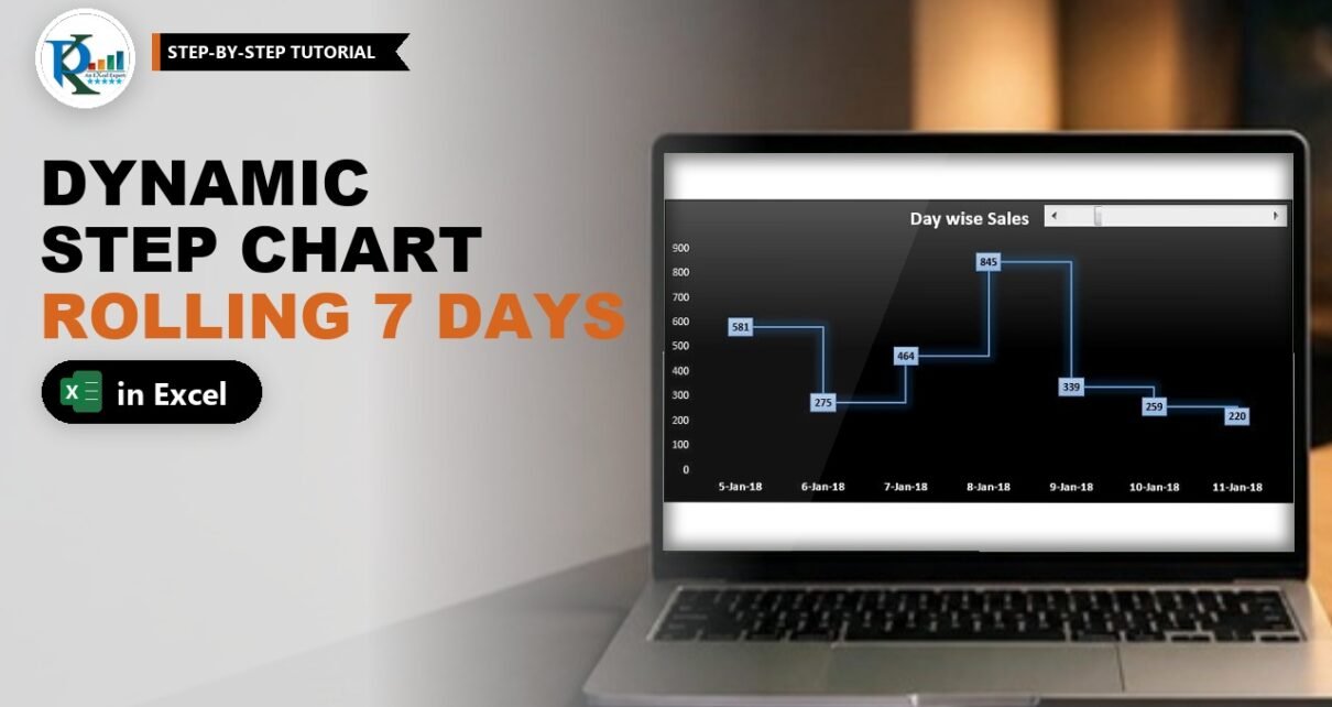
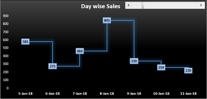
A dynamic step chart in Excel shows how a value moves from one day to the next as clean horizontal and vertical steps, instead of the sloping lines of a normal line chart. In this tutorial you build one that shows a rolling 7-day window of daily sales: drag a scroll bar and the chart slides forward one day at a time. It uses a Form Control scroll bar, three helper columns with INDEX, VLOOKUP and ISEVEN, a line chart on a date axis and a few formatting touches. No VBA is needed.
Watch the Video Tutorial
In the video PK builds the chart on a fresh sheet: the scroll bar, the doubled-up date column, the ISEVEN trick for the sales values, the date-axis fix that turns a line into steps, and the glow and label formatting.
What You Will Build
- A step chart where each day’s value stays flat until the next day, then jumps straight up or down.
- A rolling 7-day window driven by a Form Control scroll bar linked to one cell.
- Three helper columns (Date, Sales and Data Labels) that rebuild themselves whenever the scroll bar moves.
- Clean data labels that show each day’s sales once, read from cells with the Value From Cells option.
- A dark dashboard look with a glowing line and light blue label boxes.
The Sample Data
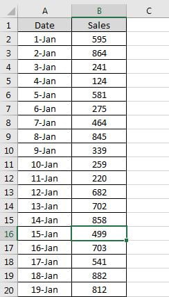
The source table is simple. Column A holds the dates (header in A1, then 1-Jan to 3-Feb, which is 34 dates) and column B holds the daily sales. The chart never plots this table directly. It plots a small helper table in columns G to I that always contains just the 7 days you have scrolled to.
Part 1 – Add the Scroll Bar
Step 1: Insert a Form Control scroll bar
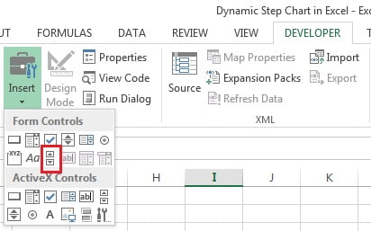
Go to Developer › Insert › Scroll Bar (Form Control) and drag it onto the sheet. If the Developer tab is missing, switch it on in File › Options › Customize Ribbon.
Step 2: Set the Format Control options
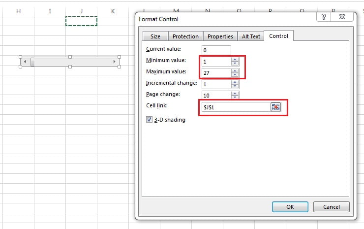
Right-click the scroll bar, choose Format Control and open the Control tab. Set:
- Minimum value: 1
- Maximum value: 27
- Incremental change: 1 (one day per click)
- Cell link:
$J$1
Why 27? There are 34 dates and the chart shows 7 at a time, so PK uses 34 – 7 = 27 as the last starting position. Cell J1 now holds a number between 1 and 27 that tells the helper table where the window starts. (See the Tips section for a small adjustment if you want the very last date to appear.)
Part 2 – Build the Step Chart Helper Columns
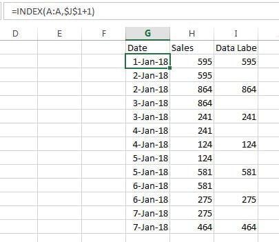
A step chart needs every date twice. The first copy carries the previous day’s value, so the line runs flat; the second copy carries the day’s own value, so the line jumps up or down on the same date. Type the headers Date in G1, Sales in H1 and Data Labels in I1.
Step 3: The Date column (G2:G14)
The first day appears once and every later day appears twice, so the 7-day window needs 13 rows:
G2       =INDEX(A:A,$J$1+1)
G3:G4    =INDEX(A:A,$J$1+2)
G5:G6    =INDEX(A:A,$J$1+3)
G7:G8    =INDEX(A:A,$J$1+4)
G9:G10   =INDEX(A:A,$J$1+5)
G11:G12  =INDEX(A:A,$J$1+6)
G13:G14  =INDEX(A:A,$J$1+7)
Press F4 while typing J1 to lock it as $J$1, then format column G as a date (Ctrl+Shift+3). The +1 skips the header row: when J1 is 1, INDEX(A:A,2) returns A2, the first date. Click the scroll bar and every date shifts by one day.
Step 4: The Sales column (H2:H14)
In H2 enter this formula and fill it down to H14:
=IF(ISEVEN(ROW()),VLOOKUP(G2,A:B,2,0),H1)How the formula works
ROW()returns the row number of the cell.ISEVENis TRUE in rows 2, 4, 6 and so on, and FALSE in rows 3, 5, 7.- In an even row,
VLOOKUP(G2,A:B,2,0)finds the date in column A and returns its real sales value. The last argument 0 forces an exact match. - In an odd row (the first copy of a new date), the formula simply repeats the value from the cell above. So on 2-Jan the first point still has 1-Jan’s 595, and the second point has 2-Jan’s own 864.
- Plotted in order, the pairs create a flat run to the new date followed by a straight jump: the step.
Step 5: The Data Labels column (I2:I14)
You only want one label per day, so copy the same formula and replace the H1 part with an empty text:
=IF(ISEVEN(ROW()),VLOOKUP(G2,A:B,2,0),"")Fill it down to I14. Even rows show the day’s value, odd rows stay blank.
Part 3 – Create and Format the Chart
Step 6: Insert a line chart
Select G1:H14 and go to Insert › Charts › Line (the plain line without markers). Because column G holds real dates, Excel normally uses a date axis, and on a date axis two points with the same date sit at the same horizontal position. That is what draws the vertical risers.
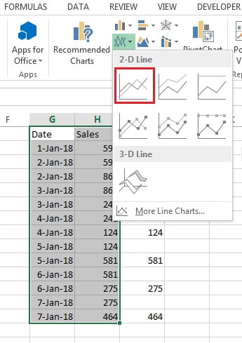
If you see sloped lines instead of steps, right-click the horizontal axis, choose Format Axis and select Date axis under Axis Type, exactly as PK shows in the video.
Step 7: Clean up and add the dark style
Use the Chart Elements (+) button to remove the gridlines and add data labels. Make the axis labels bold. Then select the whole chart and pick a black shape style from Format › Shape Styles.
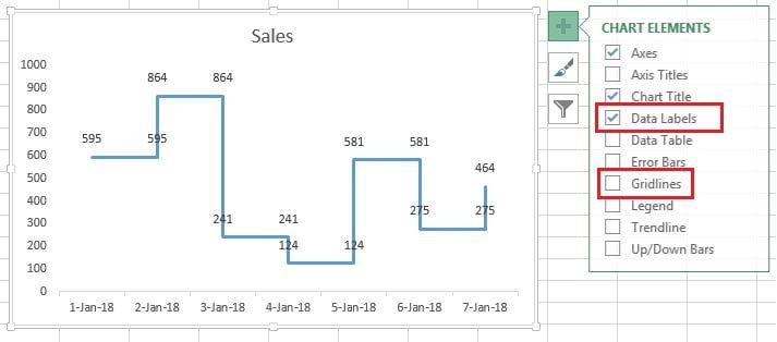
For the glowing line, right-click the line, choose Format Data Series › Effects › Glow, pick a preset and set the size to about 10 pt with a transparency of around 80 to 85 percent.
Step 8: Read the labels from column I
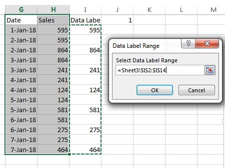
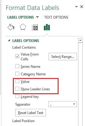
Right-click a data label and choose Format Data Labels. Tick Value From Cells, select I2:I14 and click OK. Then untick Value and Show Leader Lines, and set the Label Position to Center. Now each day shows one label at the top of its step, and the blank cells in column I hide the duplicate points.
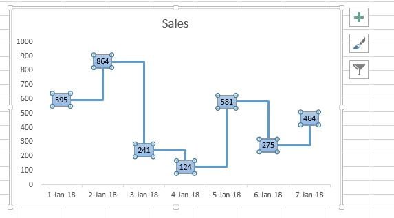
Select the labels and give them a light blue shape style from Format › Shape Styles, then set the label font colour to black so the numbers stand out on the boxes.
Step 9: Put the scroll bar on the chart
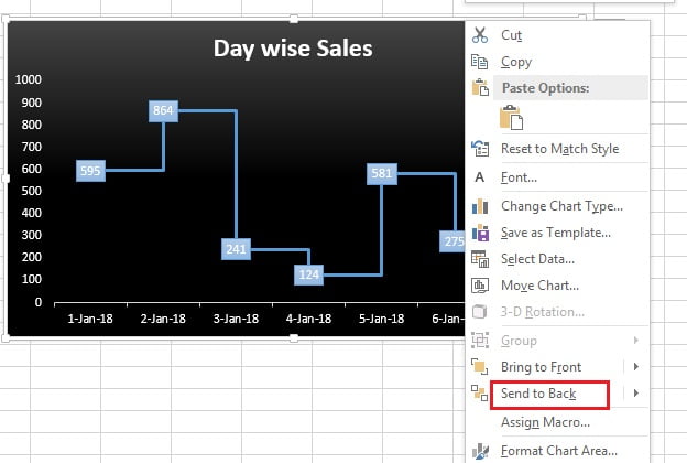
Right-click the chart area and choose Send to Back so the scroll bar stays clickable above the chart. Move the scroll bar to the top-right corner of the chart. Click its arrows and the 7-day window slides through the data.
Common Errors and Fixes
The chart shows sloped lines, not steps
The horizontal axis is a text axis, so each row gets its own slot. Open Format Axis and choose Date axis. Also check that column G holds real dates, not text.
#N/A in the Sales column
VLOOKUP cannot find the date in column A. This happens if the scroll bar maximum is larger than your data allows, or if the dates in column A are text. Lower the maximum or convert the dates.
The scroll bar cannot be clicked
The chart is sitting on top of it. Right-click the chart and choose Send to Back.
Every point shows a label
The labels still use the series values. Turn on Value From Cells with I2:I14 and untick Value.
Tips
The tips below are additions to PK’s original method.
- Reach the last date: with a start position of J1, the window shows dates J1 to J1+6. To include the final date of a 34-date list, set the maximum to 34 – 6 = 28 (number of dates minus 6).
- One formula for the whole Date column: instead of seven different INDEX formulas, enter
=INDEX(A:A,$J$1+INT((ROW()+1)/2))in G2 and fill it down to G14. It returns +1 in row 2, +2 in rows 3 and 4, and so on up to +7 in rows 13 and 14. - Change the window size: for a 10-day window, extend the helper table to 19 rows and reduce the scroll bar maximum to match.
- Use it for prices: step charts suit values that change on a date and then stay put, such as daily prices, tariffs or stock levels.
- Microsoft covers the scroll bar and other Form Controls in Overview of forms, Form controls and ActiveX controls on a worksheet.
Want It Ready-Made?
If you would rather start from the finished workbook, the Dynamic Step Chart in Excel template on NextGenTemplates.com has the scroll bar, helper table and formatting already set up. You can also browse more Excel charts and visualization templates. To go further with dynamic charts, slicers and dashboards, take the course Excel Pivot Tables and Dashboards on the NextGenTemplates Academy.
Related Tutorials
- Excel Form Controls: Combo Box, Spin Button and Option Buttons
- Excel INDEX Function: Syntax and Examples
- Excel VLOOKUP Function: Syntax, Examples and Errors
- Info-graphics with Line Chart in Excel
- Dynamic Performance Chart in Excel
Frequently Asked Questions
What is a step chart in Excel?
A step chart is a line chart that moves only horizontally and vertically. Each value stays flat until the next date and then jumps straight to the new value, which makes the exact moment of every change easy to see.
Does Excel have a built-in step chart?
No. You build it from a normal line chart by listing each date twice, so the line can run flat and then rise or fall on the same date. A date axis keeps the two points at the same horizontal position.
Why is every date repeated in the helper table?
The first copy of a date carries the previous day’s value and the second copy carries the day’s own value. Joining them gives the flat part and the vertical jump of each step.
How does the scroll bar make the chart dynamic?
The scroll bar writes a number into J1. Every INDEX formula in column G adds that number to its row offset, so changing J1 moves all 7 dates forward or back at once and the chart follows.
Why does my chart show slopes instead of steps?
The horizontal axis is set to a text axis. Right-click it, choose Format Axis and select Date axis.
Can I show more than 7 days?
Yes. Add two helper rows for every extra day and lower the scroll bar maximum by the same number of days.
About the Author
PK is a Microsoft Excel expert and trainer and the founder of PK: An Excel Expert and NextGenTemplates.com. He has been teaching Excel, Power Query and Power BI since 2016 on his YouTube channel.
Conclusion
A dynamic step chart in Excel comes down to one idea: repeat every date so the line can run flat and then jump. INDEX and the scroll bar choose the 7-day window, the ISEVEN and VLOOKUP formula fills in the right value for each point, and a date axis turns the line into clean steps. Add the glow, the light blue labels and the scroll bar on top, and you have a compact chart that is ideal for daily sales or price dashboards.