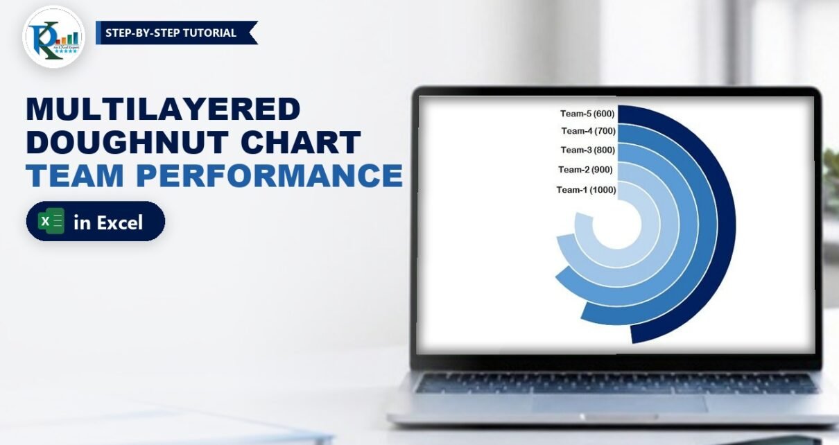
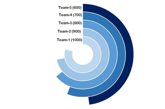
Multilayered Doughnut Chart in Excel: Team Performance Chart

A multilayered doughnut chart in Excel stacks one ring per team, so you can compare five or six teams at a glance in a dashboard or presentation. This is Part 2 of the series. In Multilayered Doughnut Chart Part 1 you built the metric-level version; here you build the team-level performance chart. Each team gets its own ring, the ring length shows its sales, and a linked label like Team-1 (1200) sits at the start of every ring. It takes one helper formula, a doughnut chart with Switch Row/Column, some fill formatting and five linked text boxes.

Multilayered doughnut chart in Excel with five blue rings for Team-1 to Team-5 and labels showing each team's sales — The finished chart: one ring per team, darkest on the outside, with the team name and sales at the start of each ring.

Table of Contents

Watch the Video Tutorial

In the video PK changes a few sales values to show the rings react, then rebuilds the chart on a new sheet: the MAX helper, the doughnut with Switch Row/Column, the No fill trick, the blue shades and the linked text box labels.

What You Will Build

Five concentric rings, one per team, built from a single doughnut chart.
Ring lengths that scale automatically from one helper formula based on the highest sales value.
Open rings: the unused part of each ring is invisible, so only the performance arc shows.
A blue colour scale from light on the inside to dark navy on the outside.
Dynamic labels such as Team-1 (1200), linked to cells so they update with the data.

Part 1 – Set Up the Data

Step 1: Enter the team sales

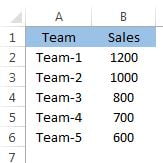
Type Team and Sales in A1:B1, then the five teams and their sales in A2:B6. PK’s example uses Team-1 to Team-5 with sales of 1200, 1000, 800, 700 and 600.

Team wise sales data with Team-1 to Team-5 in column A and sales in column B — Team-wise sales.

Step 2: Add the support column

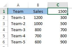
Column C holds the “rest” of each ring, the part that will be made invisible later. Enter:

C1  =MAX(B2:B6)*1.25
C2  =$C$1-B2

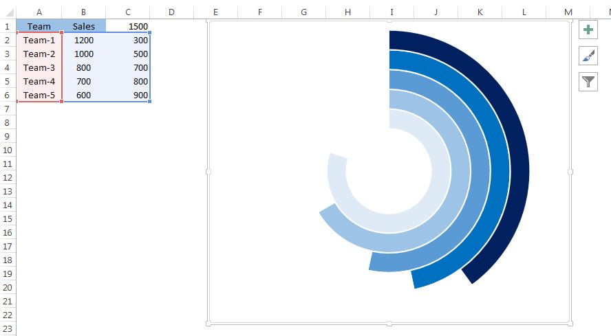
Fill C2 down to C6. With a top value of 1200, C1 returns 1500, and C2:C6 return 300, 500, 700, 800 and 900.

How the formula works

Every ring in a doughnut chart is a full circle of its own series total. Because Sales plus Rest always equals C1, every ring has the same total, so ring lengths can be compared fairly.
MAX(B2:B6)*1.25 makes the total 25 percent bigger than the best team. The top team therefore fills 1200 / 1500 = 80 percent of its ring, and there is always a gap at the end of every ring.
$C$1-B2 is the leftover for each team. C1 is locked with dollar signs so it stays fixed as you fill down.
Change any sales value and both the MAX and the leftovers recalculate, so the chart redraws itself.

Support column C with 1500 in C1 and the remaining value for each team in C2 to C6 — C1 is 125 percent of the top sales; C2:C6 hold the rest of each ring.

Part 2 – Build the Multilayered Doughnut Chart

Step 3: Insert a doughnut chart

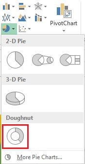
Select A2:C6 and go to Insert › Charts › Doughnut.

Insert tab chart menu with the doughnut chart option — Insert › Doughnut.

Step 4: Switch Row/Column

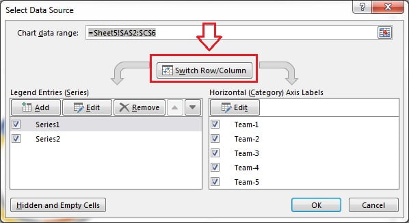
Excel first draws one ring with five slices. Right-click the doughnut, choose Select Data and click Switch Row/Column, then OK. Now every team is its own series, which means its own ring, and each ring has two slices: Sales and Rest.

Select Data Source window with the Switch Row Column button highlighted — Switch Row/Column turns each team into a ring.

Step 5: Tidy the chart and set the hole size

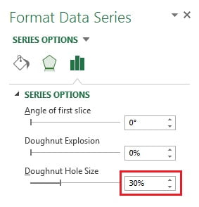
Use the + button to remove the chart title and the legend. Right-click a ring, choose Format Data Series and set the Doughnut Hole Size to 30 percent. In the Format tab give the chart area No fill and No outline, and untick Gridlines in the View tab so the chart floats on a clean sheet.

Format Data Series pane with the doughnut hole size set to 30 percent — Doughnut Hole Size 30 percent.

Step 6: Hide the Rest slices

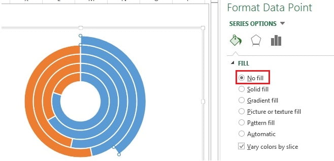
Click the orange slice of the first ring, then click it again so only that one slice is selected. In Fill & Line choose No fill. Repeat for the orange slice of every other ring. Only the sales arcs remain visible.

Orange rest slice of the first ring selected and set to No fill — Set every orange Rest slice to No fill.

Step 7: Colour the rings

Select the blue slice of each ring the same way and give it a Solid fill. PK uses a scale of blues: dark navy for the outer ring and lighter shades towards the centre.

Multilayered doughnut chart with every ring filled in a different shade of blue next to the data — Five shades of blue, dark outside and light inside.

Part 3 – Add Dynamic Labels

Step 8: Build the label text

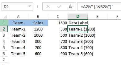
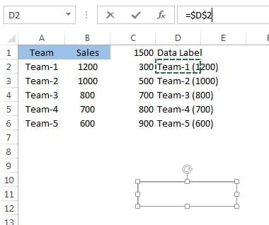
Type Data Label in D1 and enter this formula in D2, then fill it down to D6:

=A2&" ("&B2&")"

The ampersand joins the team name, a space and an opening bracket, the sales value and a closing bracket, so D2 shows Team-1 (1200).

Data Label column D with the formula joining team name and sales such as Team-1 (1200) — The label column joins name and sales.

Step 9: Link a text box to the cell

Go to Insert › Text Box and draw a small box. With the text box selected, click in the formula bar, type =$D$2 and press Enter. The box now shows the label from D2 and follows it whenever the data changes.

Text box linked to cell D2 through the formula bar — Type =$D$2 in the formula bar to link the text box.

Step 10: Format, copy and place the labels

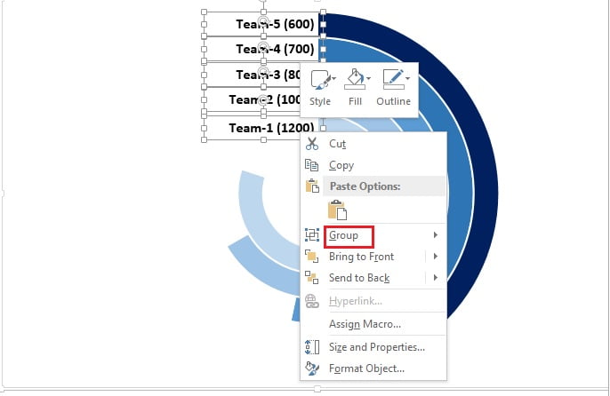
Format the text box with right alignment, Shape Fill › No fill, Shape Outline › No outline and a bold font. Team-1 is the smallest, innermost ring, so place this box at the start of that ring. Copy it four times, link the copies to D3, D4, D5 and D6, and stack them so each label sits at the start of its own ring. Select all five and use Format › Align › Align Right to line them up, then group them so they move together.

Five linked text boxes selected next to the rings with the Group option in the right-click menu — Five linked labels, aligned right and grouped.

Now type a new sales value, for example 350 for Team-1, and watch the ring and the label update together.

Common Errors and Fixes

This section and the Tips below are additions to PK’s original method.

You get one ring with five slices

The series are still in rows. Open Select Data and click Switch Row/Column.

A whole ring disappears when you set No fill

You selected the entire series. Click once to select the ring, then click the orange slice again so only that point is selected before you change the fill.

The longest ring closes into a full circle

C1 is too close to the top value, or it is a fixed number that no longer covers the data. Keep =MAX(B2:B6)*1.25 so there is always a gap.

Labels do not update

The text box holds typed text instead of a link. Select it and enter the cell reference, such as =$D$2, in the formula bar.

Tips

To show a sixth team, add it to row 7, extend the formulas to row 7, add it to the chart range and link one more text box to D7.
Change 1.25 to 1.5 for shorter, more open rings, or to 1.1 for nearly full rings. The top team always fills 1 divided by that number.
Sort the teams by sales if you want the rings to step down neatly from outside to inside.
Group the chart and the text boxes together before copying the chart into a dashboard so nothing shifts.
Microsoft’s guide Create a chart from start to finish covers Select Data and chart formatting basics.

Want It Ready-Made?

Skip the formatting and start from the finished file: get Multilayered Doughnut Chart : Part-2 from NextGenTemplates.com, or browse more Excel charts and visualization templates. If you want to build charts like this into full dashboards, the course Excel Pivot Tables and Dashboards on the NextGenTemplates Academy covers charts, infographics and dashboard design step by step.

Frequently Asked Questions

How do I make a multilayered doughnut chart in Excel?

Put each team’s sales and a Rest value in one row, insert a doughnut chart and use Switch Row/Column so every row becomes its own ring. Then set the Rest slices to No fill so only the sales arcs show.

Why multiply the maximum by 1.25?

It sets the total of every ring to 125 percent of the top sales value, so even the best team fills only 80 percent of its ring and the rings stay open and easy to compare.

What does Switch Row/Column do in a doughnut chart?

It swaps series and categories. With teams as series, each team gets its own ring instead of being a slice of a single ring.

How do I link a text box to a cell?

Select the text box, click in the formula bar, type an equals sign and the cell reference, for example =$D$2, and press Enter.

How many teams can this chart show?

Five or six rings read well. More rings get thin and the labels start to crowd.

Where is Part 1?

Part 1 builds the metric-level version of the multilayered doughnut chart. You can find it on this site as Multilayered Doughnut Chart Part 1, linked in the Related Tutorials section.

About the Author

PK is a Microsoft Excel expert and trainer and the founder of PK: An Excel Expert and NextGenTemplates.com. He has been teaching Excel, Power Query and Power BI since 2016 on his YouTube channel.

Conclusion

A multilayered doughnut chart in Excel turns a plain team sales table into a compact, eye-catching visual. One MAX formula gives every ring the same total, Switch Row/Column gives each team its own ring, No fill hides the leftovers, and linked text boxes keep the labels live. Change a number and the whole chart updates, ready for your next dashboard or presentation.

Multilayered Doughnut Chart in Excel Part 2: Team Performance

Watch the Video Tutorial

What You Will Build