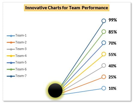
Team Level Performance Chart in Excel (Innovative Design)

This team level performance chart in Excel turns a plain list of scores into an eye-catching graphic: seven coloured lines burst out of one glowing point and end at each team’s score, like rays from a light. It is built from an ordinary Line with Markers chart, a hidden-looking helper column and a small oval shape, so it stays linked to your data and updates the moment a score changes. In this tutorial you build it step by step for seven teams and their performance scores, ready to drop into a business dashboard or a presentation slide.

Team level performance chart in Excel: seven coloured lines from one glowing black point ending at 10, 25, 40, 55, 70, 85 and 99 percent — The finished chart: every team is one line from a shared start point to its performance score.

Table of Contents

Watch the Video Tutorial

In the video, PK adds a zero Start Point column, inserts a Line with Markers chart, switches rows and columns so each team becomes its own line, then formats the markers and labels and places a glowing oval at the start point.

What You Will Build

A chart where each of seven teams is drawn as its own coloured line.
All lines start from one point and end at the team’s performance score.
Large hollow markers with bold percentage labels at the end of every line.
A legend on the left that lists Team-1 to Team-7.
A glowing oval that hides the start point and gives the chart its signature look.

Part 1 – Prepare the Data for the Team Performance Chart

Step 1: Enter the team scores

Type the team names in column A and their scores in column C, formatted as percentages:

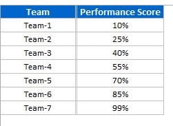
Team wise performance score table for the Excel chart: Team-1 10% up to Team-7 99% — The source data: one performance score per team.

You can replace the team names with real names and use any other KPI in place of the performance score.

Step 2: Add a Start Point helper column

Every line needs two points: where it starts and where it ends. Put a helper column between the team names and the scores. Type Start Point in B1 and 0 in B2:B8, so the layout is:

        A         B             C
1       Team      Start Point   Performance Score
2       Team-1    0             10%
3       Team-2    0             25%
4       Team-3    0             40%
5       Team-4    0             55%
6       Team-5    0             70%
7       Team-6    0             85%
8       Team-7    0             99%

Why not hide column B? By default Excel does not plot data from hidden columns, so a hidden Start Point column would disappear from the chart. Instead, make column B very narrow so it is out of the way but still visible to the chart.

Part 2 – Build the Line Chart

Step 3: Insert a Line with Markers chart

Select A1:C8 and go to Insert > Charts > Line > Line with Markers. Turn off the sheet gridlines from View > Gridlines so the chart sits on a clean background.

At first the chart looks wrong: you get two lines, one called Start Point that runs flat along zero and one called Performance Score that climbs across the seven teams. That is because Excel treats each column as a series.

Step 4: Remove the axes and gridlines

Click the vertical axis and press Delete, then do the same for the horizontal axis and the chart gridlines. The chart only needs the lines themselves.

Step 5: Switch Row/Column

Right-click the chart, choose Select Data and click Switch Row/Column, then OK. Now each row becomes a series. Clicking the Team-7 line shows this series formula in the formula bar:

=SERIES(Sheet1!$A$8,Sheet1!$B$1:$C$1,Sheet1!$B$8:$C$8,7)

How the series works

$A$8 is the series name, Team-7, which also appears in the legend.
$B$1:$C$1 gives the two category labels, Start Point and Performance Score, so each line has exactly two points.
$B$8:$C$8 holds the values: 0 for the start and 99% for the end.
All seven lines share the same first point (0), which is why they fan out from one spot. A higher score gives a steeper, longer line.

Step 6: Move the legend to the left

Right-click the legend, choose Format Legend and set the position to Left. Then resize the chart so it is taller than it is wide, which makes the fan of lines look more dramatic.

Part 3 – Format Lines, Markers and Labels

Step 7: Format each line and its markers

Double-click the first line to open the format pane, then set:

Fill & Line > Line: width about 1.5 pt.
Marker > Marker Options: Built-in, size 10 instead of 5.
Marker > Fill: Solid fill, white.
Marker > Border: keep the automatic colour and set the width to 1.5 pt.

The white fill with a coloured border creates the hollow ring at the end of each line. Repeat the same settings for all seven lines.

Step 8: Add data labels

Click the end marker of a line, right-click and choose Add Data Label. In Format Data Labels keep Value ticked and set the Label Position to Right. In the video the label font is Lato Black at about size 10 to 11. Do this for each line; to speed it up, format one label and use the Format Painter to copy the style to the others.

Because the labels show the real cell values, typing a new score in column C moves both the line end and the label. In the video PK changes Team-1 from 10% to 5% and the chart redraws instantly.

Part 4 – Add the Glowing Start Point

Step 9: Insert and style an oval

Go to Insert > Shapes > Oval and draw a small circle over the point where all the lines meet. On the Format tab pick a black shape style, then open Shape Effects > Glow and choose a glow variation. The glowing black ball hides the start point and makes the lines look like rays.

Step 10: Group and add a title

Select the chart and the oval together and group them, so they move and resize as one object. Finally add a title such as Innovative Charts for Team Performance.

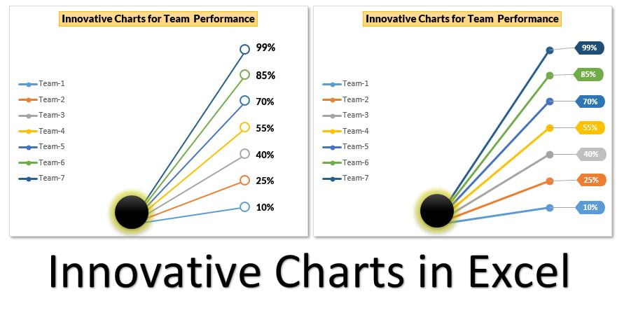
Two versions of the innovative team performance chart in Excel, one with hollow markers and one with coloured tag labels — Two versions from the same data: hollow ring markers (left) and coloured tag labels (right).

The second version on the right uses the same chart with filled markers and coloured label boxes in each team’s colour. It is shown in the video’s introduction and included in the ready-made template.

Common Errors and Fixes

Only two lines appear instead of seven. Excel is still plotting by column. Use Select Data > Switch Row/Column.
The lines do not start from the same point. The Start Point column is hidden or missing. Unhide it and make it narrow, or check that every row has 0 in column B.
Labels appear at both ends of a line. You added labels to the whole series. Delete the labels at the start point, or add the label only to the end marker. (Addition)
The oval drifts away when the chart is moved. The shape is not grouped with the chart. Select both and group them. (Addition)

Tips

Sort the teams by score so the lines fan out in order and the labels never overlap. (Addition)
If you prefer to hide column B, go to Select Data > Hidden and Empty Cells and tick Show data in hidden rows and columns. (Addition, not in the video)
Keep the chart to about seven to ten teams; more lines crowd the labels. (Addition)
Use colours that match your dashboard theme by changing the line colours, and the markers follow automatically.
For the basics of building and editing charts, see Microsoft’s Create a chart from start to finish.

Want It Ready-Made?

If you would rather start from the finished file with both chart versions, get An Innovative Chart for Team Level Performance on NextGenTemplates.com, or browse more Excel chart templates. To build charts like this and complete dashboards with confidence, join Excel Pivot Tables and Dashboards on NextGenTemplates Academy.

Frequently Asked Questions

What chart type is used for this team performance chart?

It is a standard Line with Markers chart. Switching rows and columns turns every team into its own two-point line, from a shared start value of zero to the team’s score.

Why do I need the Start Point column?

Each line needs a beginning and an end. The Start Point column gives every team the same first value, zero, so all the lines begin at one spot and fan out to their scores.

Can I hide the helper column?

Excel does not plot hidden columns by default, so the chart would lose its start point. Make the column narrow instead, or enable the option to show data in hidden rows and columns.

Does the chart update when the scores change?

Yes. The lines and the labels read directly from the cells, so typing a new score immediately moves the line and its percentage label.

Can I use it for KPIs other than performance score?

Yes. Any percentage or score per team, region or product works, such as target achievement, quality score or customer satisfaction.

About the Author

PK is a Microsoft Excel expert and trainer and the founder of PK: An Excel Expert and NextGenTemplates.com. He has been teaching Excel, VBA, Power Query and Power BI since 2016 on his YouTube channel.

Conclusion

A team level performance chart in Excel like this one needs no add-ins: a zero Start Point column, a Line with Markers chart switched to one series per team, white hollow markers with value labels, and a glowing oval at the start. It stays fully linked to your data, so it is just as useful in a monthly dashboard as it is in a one-off presentation. Build it once, then swap in your own teams and KPI.

Innovative Chart for Team Level Performance in Excel

Watch the Video Tutorial

What You Will Build