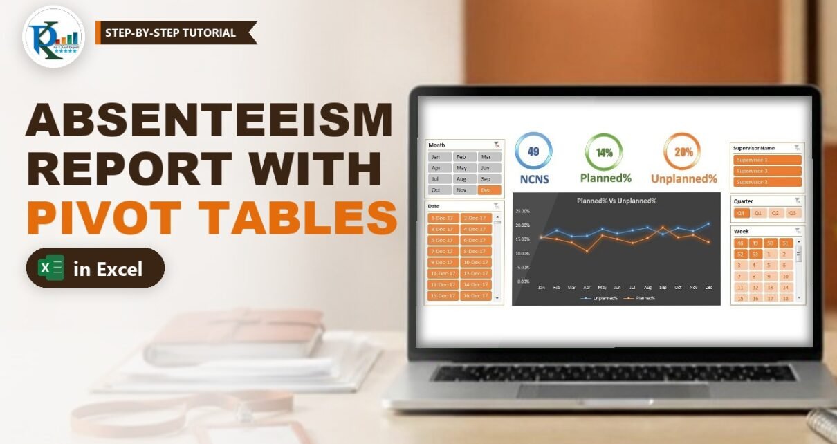
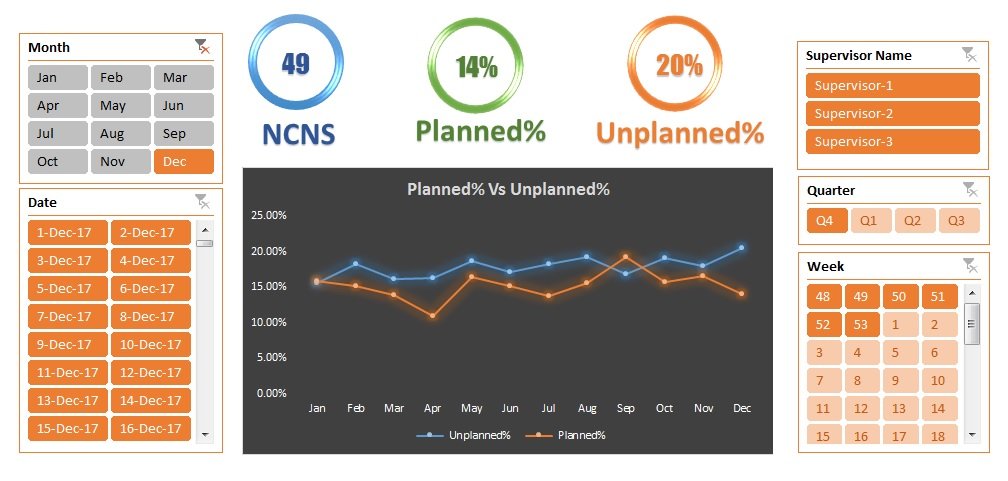
An absenteeism report in Excel shows at a glance how much of your team’s scheduled time was lost to unplanned absence and how much went to planned leave. In this tutorial you build PK’s process absenteeism report: a daily raw data sheet, a dynamic pivot range, three calculated fields (Scheduled, Unplanned% and Planned%), traffic-light icons against 12% and 15% targets, and a summary page with slicers, KPI circles and a line chart. No VBA is needed.
Watch the Video Tutorial
Part 1 prepares the raw data, the dynamic range and the calculated fields:
Part 2 formats the pivot, adds the icons, copies the report sheets and builds the chart:
Part 3 adds the KPI circles, slicers, Index page and Back buttons:
What You Will Build
- A Raw_Data sheet with one row per employee per day and 1/0 helper columns.
- An error check that turns the header red when a wrong attendance code is typed.
- A dynamic pivot range built with OFFSET and COUNTA.
- Three calculated fields with red and green icons against your targets.
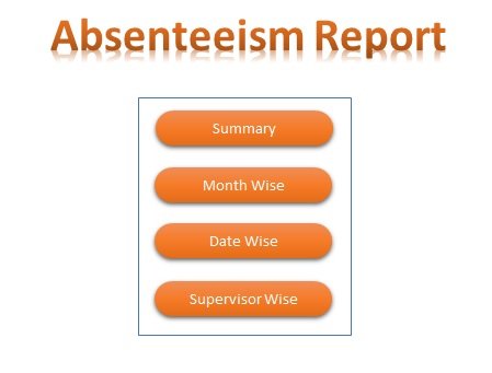
- Four report sheets (Summary, Month Wise, Date Wise, Supervisor Wise) linked from an Index page.
How the Absenteeism Report in Excel Is Laid Out
The workbook has an Index page, a Summary dashboard, three pivot reports, the Raw_Data sheet and a hidden Support sheet that feeds the dashboard.
The attendance codes
- P – present.
- WO – week off.
- L – planned leave, already marked in the roster.
- A – absent. The employee informed the supervisor, but the day was not leave in the roster, so it is unplanned.
- NCNS – no call, no show. Nobody was informed, so it is always unplanned.
If your process uses other codes, just change the helper headers to match.
Part 1 – Prepare the Raw Data
Step 1: Enter one row per employee per day
Raw_Data has the columns Date, Week, Month, Quarter, Year, EMP Name, Supervisor Name, Shift and Attendance. The sample holds 20 employees for every day of 2017 (7,300 rows). Week, Month and Year are formulas:
B2  =WEEKNUM(A2)
C2  =TEXT(A2,"MMM")
E2  =YEAR(A2)
Step 2: Add the helper columns
Type the five codes as headers in J1:N1 (WO, NCNS, A, L, P) in a different header colour, because they are formulas. In J2 enter the formula below, fill it right to N2 and then down:
J2 =COUNTIF($I2,J$1)How the formula works
$I2locks the column, so every helper cell looks at the Attendance column of its own row.J$1locks the row, so each cell compares against its own header.- COUNTIF on one cell is a match test that returns 1 or 0. The pivot then sums these 1s to count each code.
Step 3: Add a Check column and a red-header warning
In O1 type Check and in O2 enter =SUM(J2:N2). A valid row always returns 1; a row with a wrong code returns 0. Select the header row A1:O1, go to Home > Conditional Formatting > New Rule > Use a formula to determine which cells to format and enter:
=COUNTIF($O:$O,0)>0Pick a red fill. When any row has a Check of 0, the header turns red; filter column O for 0 to find and fix it.
Part 2 – Make the Pivot Range Dynamic
Step 4: Create the Pivot_Range name
Go to Formulas > Name Manager > New, name it Pivot_Range and use:
=OFFSET(Raw_Data!$A$1,,,COUNTA(Raw_Data!$A:$A),COUNTA(Raw_Data!$1:$1))OFFSET starts at A1. Its height is the count of filled cells in column A and its width the count of headers in row 1, so the range grows with your data.
Step 5: Point the pivot table at the name
Insert a pivot table, go to PivotTable Analyze > Change Data Source, clear the fixed range, press F3 and pick Pivot_Range. Now new rows only need a Refresh.
Part 3 – Calculated Fields for Planned and Unplanned Absenteeism
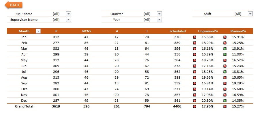
Put Month in Rows and the sums of P, NCNS, A and L in Values. Then add three fields from PivotTable Analyze > Fields, Items & Sets > Calculated Field:
Scheduled   = P + A + NCNS
Unplanned%  = (A + NCNS) / Scheduled
Planned%    = L / (Scheduled + L)
How the formula works
- Scheduled is everyone rostered to work: those who came (P) plus those expected who did not (A and NCNS).
- Unplanned% divides the unplanned absences by Scheduled.
- Planned% divides leave by Scheduled + L, because people on leave are not in the scheduled count.
- Calculated fields work on the totals, so every subtotal and the Grand Total are correct too.
With the sample data, January has P 312, NCNS 41, A 17 and L 70. Scheduled is 370, Unplanned% is 58 / 370 = 15.68% and Planned% is 70 / 440 = 15.91%.
Part 4 – Format the Pivot and Add Traffic Lights
Step 6: Clean up the pivot
- Set Unplanned% and Planned% to Percentage, 2 decimal places.
- In PivotTable Options: show blank for error values, set report filter fields per column to 2 and untick Autofit column widths on update. On the Data tab set items to retain per field to None.
- Pick a pivot style (the file uses PivotStyleMedium3), switch to Tabular Form and turn off gridlines and headings.
Step 7: Icon sets against the 12% and 15% targets
Select the Unplanned% values and go to Conditional Formatting > New Rule. Choose All cells showing “Unplanned%” values so the rule follows the pivot. Pick Icon Sets with traffic lights, set both Type boxes to Number and the value to 0.12: red when the value is 0.12 or more, green otherwise. Repeat for Planned% with 0.15.
Part 5 – Date Wise and Supervisor Wise Reports
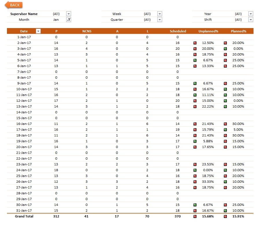
Rename the finished sheet Month Wise and add filters for EMP Name, Supervisor Name, Quarter, Year and Shift. Then copy the sheet (right-click the tab > Move or Copy > Create a copy):
- Date Wise: put Date in Rows and Month in the filters, so you can pick a month and see every day.
- Supervisor Wise: put Supervisor Name and then EMP Name in Rows for a subtotal per supervisor and a line per employee.

Part 6 – The Summary Dashboard
Step 8: The month-on-month line chart
Copy Month Wise again as Support. Keep only Unplanned% and Planned% and turn off the grand total (PivotTable Options > Totals & Filters). Insert a line chart, hide the field buttons, put the legend at the bottom, title it Planned% Vs Unplanned%, pick a dark style and remove the gridlines. Cut it to a new Summary sheet.
Step 9: The three KPI circles
On Support, add a second pivot with the totals of NCNS, Unplanned% and Planned%, and pull the numbers into fixed cells with GETPIVOTDATA (type = and click the pivot cell, and Excel writes it for you):
Q2  =GETPIVOTDATA(" NCNS",$G$5)
Q3  =GETPIVOTDATA(" Planned%",$G$5)
Q4  =GETPIVOTDATA(" Unplanned%",$G$5)
On Summary, draw a Donut shape, thin the ring with its yellow handle and apply Shape Effects > Preset 5 with no shadow. Add a text box in the middle and type =Support!Q2 in the formula bar to link it. Copy the circle for Planned% (=Support!Q3) and Unplanned% (=Support!Q4) and add a WordArt label under each.
Step 10: Slicers
Select the KPI pivot on Support, go to PivotTable Analyze > Insert Slicer and tick Date, Week, Month, Quarter and Supervisor Name. Cut them to Summary and set their columns (four for Quarter). Every slicer click now updates the circles.
Part 7 – Index Page and Back Buttons
Add an Index sheet with four rounded rectangles (Summary, Date Wise, Month Wise, Supervisor Wise), lined up with Align Center and Distribute Vertically. Select each one, press Ctrl+K, choose Place in This Document and pick its sheet. Add a BACK arrow on every report linked to Index, then hide Support.
Common Errors and Fixes
The header row turned red
A row has a code outside WO, NCNS, A, L and P. Filter column O for 0 and fix it.
#DIV/0! in Unplanned% or Planned%
Nothing was scheduled, so the field divides by zero. Show blank for error values, as in Step 6.
New rows do not appear in the report
Make sure the source is Pivot_Range and column A has no blank cells inside the data, then press Data > Refresh All.
The icons do not cover new rows
The rule was applied to selected cells only. Edit it and switch to All cells showing “Unplanned%” values.
Tips
- Change 0.12 and 0.15 in the icon rules to your own process targets.
- The sample types the Quarter by hand.
="Q"&ROUNDUP(MONTH(A2)/3,0)returns Q1 to Q4 if you prefer a formula (an addition, not in the original file). - The slicers drive the KPI pivot only. To filter other pivots too, right-click a slicer and use Report Connections (an addition).
- Microsoft’s guide to calculating values in a PivotTable covers calculated fields in detail.
Want It Ready-Made?
If you would rather start with the finished workbook, the Absenteeism Report in Excel template on NextGenTemplates.com has every sheet from this tutorial ready for your own data. For a wider set of people reports there is the HR & Workforce Analytics Bundle, or browse all HR and payroll Excel templates. To master pivot tables, slicers, pivot charts and dashboards step by step, join the video course Excel Pivot Tables and Dashboards.
Related Tutorials
- Conditional Formatting in a Pivot Table with 3 Examples
- 10 Useful Pivot Table Tips
- Stylish Pivot Chart with Slicer in Excel
- Attendance Sheet in Excel: 7 Methods Compared
- Excel OFFSET Function for Dynamic Ranges
Frequently Asked Questions
How do you calculate the absenteeism rate in Excel?
In this report the unplanned absenteeism rate is (A + NCNS) divided by Scheduled, where Scheduled is P + A + NCNS. Add it as a pivot table calculated field so it is worked out from the totals of each month, date or supervisor.
What is the difference between planned and unplanned absenteeism?
Planned absence is leave already marked in the roster (L). Unplanned absence is anything the roster did not expect: A, where the employee informed the supervisor on the day, and NCNS, where nobody was informed.
Why does Planned% divide by Scheduled plus L?
Employees on planned leave are not part of the scheduled count. Adding L back to the denominator measures leave against everyone who could have been rostered.
How do I add new days to the absenteeism report?
Paste the new rows under the data in Raw_Data, fill the helper formulas down and click Refresh All. The OFFSET-based Pivot_Range name picks up the new rows automatically.
Do I need VBA for this report?
No. It uses formulas, a named range, pivot tables, calculated fields, conditional formatting, slicers, shapes and hyperlinks only.
About the Author
PK is a Microsoft Excel expert and trainer and the founder of PK: An Excel Expert and NextGenTemplates.com. He has been teaching Excel, Power Query and Power BI since 2016 on his YouTube channel.
Conclusion
An absenteeism report in Excel does not need complex formulas. COUNTIF helper columns, a dynamic OFFSET range and three calculated fields give you Scheduled, Unplanned% and Planned% for any month, date or supervisor. Add traffic-light icons, a line chart, slicers and an Index page, and your team gets a report that updates with one refresh.