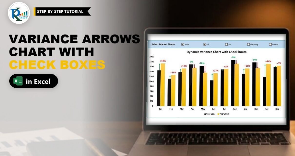
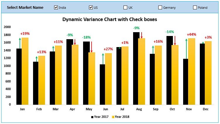
A dynamic variance arrows chart with check boxes shows this year against last year for every month and puts a green up arrow or a red down arrow on top of each pair of columns, with the percentage change written beside it. Tick one or more market check boxes and the whole chart recalculates for just those markets. In this tutorial you build it from a plain sales table with SUMIFS, two error-bar helper columns and Form Control check boxes. No VBA is needed, and it works in Excel 2013 and later.
Watch the Video Tutorial
PK builds the chart from a blank workbook: check boxes, SUMIFS formulas, error-bar arrows and percentage labels.
What You Will Build
- A clustered column chart with black columns for 2017 and gold columns for 2018, month by month.
- Green up arrows and red down arrows drawn with custom error bars, sized exactly to the change between the two years.
- Percentage labels such as +19% and -9% pulled from cells with Value From Cells.
- Five market check boxes (India, US, UK, Germany and Poland). Tick any combination and the chart adds those markets together.
The Sales Data
Everything starts from one flat table on a sheet called Data: Market Name (A), Year (B), Month (C) and Sales (D), for five markets, 2017 and 2018, and twelve months.
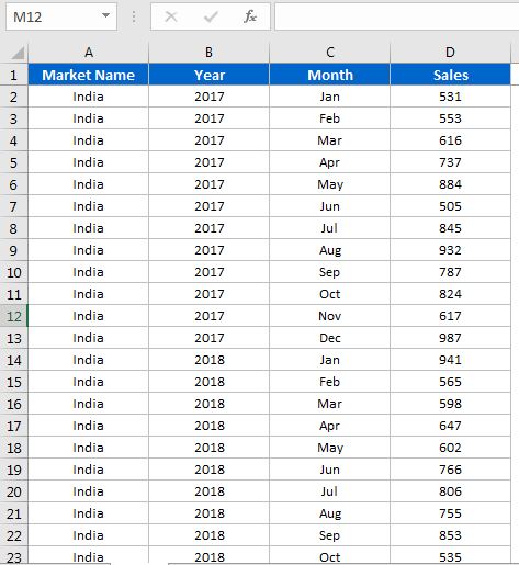
Add two more sheets: Support for the helper calculations and Chart for the final dashboard. On the Chart sheet, turn off gridlines (View → untick Gridlines) so the chart sits on a clean background.
Part 1: Add the Market Check Boxes
Step 1: Set up the Support sheet
On the Support sheet type Month in A1 and Jan to Dec in A2:A13 (type Jan and drag the fill handle down). Put Year 2017 in B1 and Year 2018 in C1.
Step 2: List the unique market names
Copy the Market Name column from the Data sheet, paste it into column Q of the Support sheet with Paste Special → Values, then use Data → Remove Duplicates. You are left with India, US, UK, Germany and Poland in Q1:Q5.
Step 3: Insert five Form Control check boxes
Go to the Chart sheet and choose Developer → Insert → Check Box (Form Control). Draw the first one and rename it India. Copy and paste it four times and rename the copies US, UK, Germany and Poland. Select all five and use Format → Align → Align Top and then Distribute Horizontally so they sit in a neat row.
Step 4: Link each check box to a cell
Right-click the India check box, choose Format Control, and in the Cell link box click Support!R1, the cell beside India. R1 now shows TRUE when India is ticked and FALSE when it is not. Repeat for the other four: US to R2, UK to R3, Germany to R4 and Poland to R5. The order must match the names in Q1:Q5.
Part 2: Sum Sales for the Ticked Markets
Step 5: The 2017 formula
In Support!B2 enter this formula (it is one formula, split over lines here so you can read it):
=IF($R$1,SUMIFS(Data!D:D,Data!A:A,Support!$Q$1,Data!C:C,Support!A2,Data!B:B,2017),0)
+IF($R$2,SUMIFS(Data!D:D,Data!A:A,Support!$Q$2,Data!C:C,Support!A2,Data!B:B,2017),0)
+IF($R$3,SUMIFS(Data!D:D,Data!A:A,Support!$Q$3,Data!C:C,Support!A2,Data!B:B,2017),0)
+IF($R$4,SUMIFS(Data!D:D,Data!A:A,Support!$Q$4,Data!C:C,Support!A2,Data!B:B,2017),0)
+IF($R$5,SUMIFS(Data!D:D,Data!A:A,Support!$Q$5,Data!C:C,Support!A2,Data!B:B,2017),0)
Fill it down to B13. PK writes the first IF block, then pastes it four times, changing only the 1 in $R$1/$Q$1 to 2, 3, 4 and 5.
How the formula works
SUMIFS(Data!D:D, ...)adds the Sales column where the market equals the name in Q1, the month equals the month in A2 and the year equals 2017.IF($R$1, ..., 0)only keeps that total when the India check box is ticked (R1 is TRUE). Otherwise it adds 0.- The five IF blocks are added together, so ticking India and US gives India plus US, and ticking all five gives the total of every market.
Step 6: The 2018 formula
Copy B2:B13 to C2:C13. Then, with C2:C13 selected, press Ctrl+H and replace 2017 with 2018. Only the selection is searched, so column B stays on 2017.
Part 3: Helper Columns for the Variance Arrows
The arrows are error bars on two invisible series. Add four helper columns to the Support sheet:
| Column | Header | Formula in row 2 |
|---|---|---|
| D | Max Left | =MAX(B2:C2) |
| E | Max Right | =D2 |
| F | Up Error Bar | =IF(C2>B2,C2-B2,NA()) |
| G | Down Error Bar | =IF(C2<B2,B2-C2,NA()) |
Fill all four down to row 13. With India and US ticked, January goes from 1455 to 1731, so the Up Error Bar is 276; April falls from 1690 to 1543, so its Down Error Bar is 147.
Why these helpers work
Max Left and Max Right sit at the height of the taller column. A minus error bar of the size of the change runs from there down to the shorter column. NA() matters: a #N/A error amount draws no error bar, so each month gets only one arrow.
Part 4: Build the Variance Arrows Chart with Check Boxes
Step 7: Insert the column chart
Select Support!A1:E13 and choose Insert → 2-D Clustered Column. Right-click the chart, choose Select Data, and use the arrows to move Max Left to the top, so the order is Max Left, Year 2017, Year 2018, Max Right.
Step 8: Add custom error bars
Select the Max Left series, click the + (Chart Elements) button and tick Error Bars. Do the same for Max Right. Then select the Max Left error bars and in Format Error Bars set:
- Direction: Minus
- End Style: No Cap
- Error Amount: Custom → Specify Value, Negative Error Value =
=Support!$F$2:$F$13(the Up Error Bar column)
Give the Max Right error bars the same settings, with the Negative Error Value set to =Support!$G$2:$G$13 (the Down Error Bar column).
Step 9: Hide the helper columns and draw the arrows
Set Max Left and Max Right to Fill → No fill, so only their error bars remain. Then format the error-bar lines:
- Max Left error bars: Solid line, green, width 1.5 pt, and a Begin Arrow type. This gives the up arrow.
- Max Right error bars: Solid line, red, width 1.5 pt, and an End Arrow type. This gives the down arrow.
Step 10: Secondary axis, overlap and colours
Open Format Data Series for Max Left and choose Secondary Axis, then do the same for Max Right. Set Series Overlap to about 20 to 25% and Gap Width to about 75% on both the primary series (2017) and the secondary series. Fill the Year 2017 series with solid black and Year 2018 with solid gold.
Step 11: Clean up
Delete the secondary vertical axis, click the Max Left and Max Right legend entries one at a time and press Delete, and untick Gridlines. The legend now shows only Year 2017 and Year 2018.
Part 5: Add the Percentage Labels
Step 12: Label helper columns
Add two more columns. In H1 type Up Data Label and in H2:
=IF(ISERROR(F2),"","+"&TEXT(F2/B2,"0%"))In I1 type Down Data Label and in I2:
=IF(ISERROR(G2),"","-"&TEXT(G2/B2,"0%"))Fill both down to row 13. The change is divided by the 2017 value because last year is the base. TEXT(...,"0%") turns 0.19 into 19%, and the plus or minus sign is joined in front, so you get +19% and -9%. ISERROR returns an empty string for months where that arrow does not exist.
Step 13: Link the labels with Value From Cells
Select the Max Left series. Because it has no fill it can be hard to click, so use Format → Current Selection and pick Series “Max Left” from the drop-down. Right-click, Add Data Labels, then open Format Data Labels, tick Value From Cells, select Support!H2:H13, and untick Value and Show Leader Lines. Make the labels green, bold and a little larger from the Home tab.
Repeat for Max Right with Support!I2:I13 and colour those labels red.
Step 14: Move the chart to the dashboard
Cut the chart (Ctrl+X) and paste it on the Chart sheet under the check boxes. Add a light rectangle behind them (Send to Back), then select everything and Group it. Tick a few markets and watch the columns, arrows and percentages update.
Modern Excel Alternative
This section is an addition and is not shown in the video. In Excel 365 and 2021 you can replace the five IF blocks with one formula that reads the check-box cells directly:
=SUM(SUMIFS(Data!$D:$D,Data!$A:$A,FILTER($Q$1:$Q$5,$R$1:$R$5),Data!$C:$C,A2,Data!$B:$B,2017))FILTER returns only the ticked market names, SUMIFS returns one total per market, and SUM adds them. If no box is ticked, FILTER returns an error, so wrap the formula in IFERROR(…,0) if you want 0 instead.
Common Errors and Fixes
The arrows sit beside the columns instead of on them
Max Left and Max Right must be on the secondary axis, and the overlap and gap width need to be similar on both axes. Also check the series order in Select Data: Max Left first, Max Right last.
Every month shows two arrows
The error-bar helper must return NA(), not 0 or an empty string, when that direction does not apply. Check columns F and G.
The chart shows zero for every month
No box is ticked, or a box is linked to the wrong cell. Check that the links run R1 to R5 in the same order as Q1:Q5.
Tips
- If only one market should show at a time, option buttons are simpler than check boxes.
- Prefer to filter with a stylish slicer instead? The dynamic variance arrows chart with slicers builds the same chart and connects it to a slicer.
- Microsoft’s guide on how to add, change or remove error bars in a chart explains every error-bar option used here.
Want It Ready-Made?
If you want the finished workbook with the check boxes, formulas and formatting already done, get the Dynamic Variance Arrows Chart with Check Boxes template on NextGenTemplates.com, or browse more Excel templates. To learn charts, slicers and complete dashboards step by step, see the course Excel Pivot Tables and Dashboards.
Related Tutorials
- Dynamic Variance Arrows Chart with Slicers (Part 2)
- Excel Form Controls: Combo Box, Spin Button and Option Buttons
- How to Add a Checkbox in an Excel Table
- Target vs Actual Sales Dynamic Chart
- Yesterday vs Today Sales Chart
Frequently Asked Questions
How are the variance arrows drawn in an Excel chart?
They are custom minus error bars on two invisible column series that sit at the height of the taller column. The error amount equals the change between the years, and the line uses an arrow head, green for up and red for down.
Why use check boxes instead of option buttons?
Option buttons allow only one choice. Check boxes let you tick several markets at once, and the SUMIFS formula adds every ticked market together.
How do I show the percentage change on the chart?
Calculate the label text in a helper column with the TEXT function, add data labels to the invisible series and use Value From Cells to point the labels at that column. Step 12 shows both formulas.
Which Excel version do I need?
Excel 2013 or later, because Value From Cells for data labels was introduced in Excel 2013. The formulas and error bars also work in Excel 2010.
About the Author
PK is a Microsoft Excel expert and trainer and the founder of PK: An Excel Expert and NextGenTemplates.com. He has been teaching Excel, Power Query and Power BI since 2016 on his YouTube channel.
Conclusion
A dynamic variance arrows chart with check boxes turns a flat sales table into a year-on-year story your audience reads in seconds. Linked check boxes feed SUMIFS, two helper series carry error bars shaped as arrows, and Value From Cells adds the percentages. Build it once on the Support sheet, group it on a clean dashboard, and every tick of a market check box updates the columns, arrows and labels together.