Part of the free Module 4: Sort and Filter · Lesson 1 of 11 · Full Excel course
Updated on 5 September 2026 · Works in Excel 365, 2021, 2019 and 2016 unless noted.
To sort data in Excel, click one cell inside your table, go to Data > Sort & Filter and choose A to Z, Z to A or the Sort dialog. Excel reorders whole rows, keeps every cell in its row and can nest up to 64 levels, so you can sort by Region, then Salesperson, then Date in one pass.
What sorting does and when to use it
A sort rearranges complete rows so that one column runs in a chosen order: smallest to largest, A to Z, oldest to newest, or a custom sequence such as Low, Medium, High. Every other cell in the row travels with it, so a sales figure never separates from its date or its salesperson. Excel can sort by cell values, cell colour, font colour or conditional formatting icon.
Sort before you scan for the largest orders, before you remove duplicates, before you build running totals, and whenever a report should read in a predictable order. If you also need the original order back later, add a serial number column first; sorting by that column restores the data at any time.
The sample data
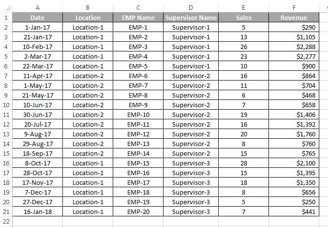
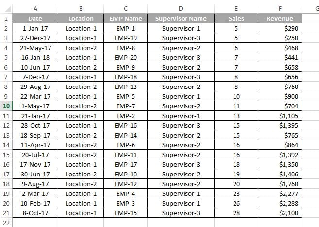
The table below records daily sales by Date, Location, Supervisor, Employee and Sales. It has one header row and no blank rows or columns, which is the structure Excel needs to detect the whole range automatically. Download the same data from the course practice file.
How to sort one column with the filter drop-down
- Click any cell inside the data.
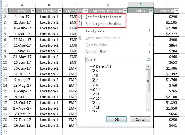
- Press Ctrl+Shift+L, or go to Data > Sort & Filter > Filter, to switch on the AutoFilter arrows.
- Open the drop-down arrow on the Sales header.
- Click Sort Smallest to Largest. For text columns the options read Sort A to Z; for dates they read Sort Oldest to Newest.
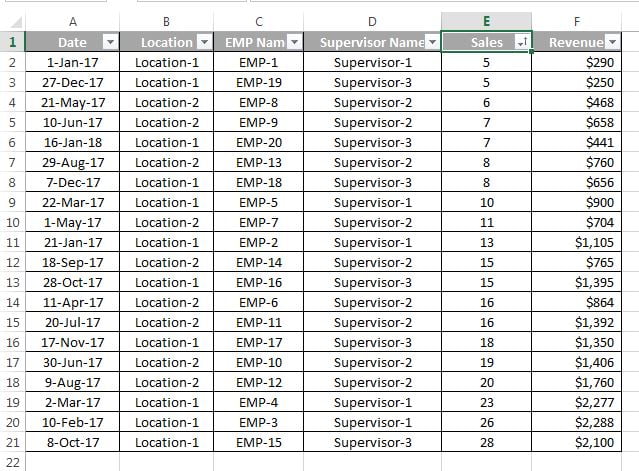
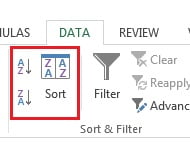
The whole table is reordered by Sales in ascending order, and a small arrow appears on the Sales filter button to show which column is sorted. The two quick buttons on the Data tab, A to Z and Z to A, do the same job without switching the filter on; they sort by whichever column the active cell is in.
How to run a multi-level sort with the Sort dialog
The goal is to order the rows by Sales, then by Location within equal sales, then by Date within equal locations.
- Click any cell in the data and go to Data > Sort & Filter > Sort. The keyboard route is Alt, A, S, S.
- In the first level choose Sales under Sort by, keep Cell Values under Sort On and set Order to Smallest to Largest.
- Click Add Level, choose Location and set Order to A to Z.
- Click Add Level again, choose Date and set Order to Oldest to Newest.
- Make sure My data has headers is ticked so the header row stays at the top, then click OK.
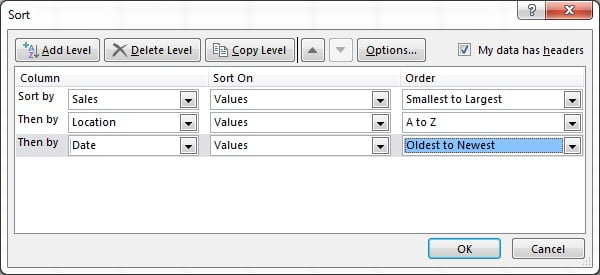
The result is ordered first by Sales; where two rows share the same sales figure they are ordered by Location, and where the location also matches, by Date. Use the up and down arrows in the dialog to change the priority of a level, Copy Level to duplicate one, and Delete Level to remove one.
Sort commands compared
| Method | Where | Best for | Levels |
|---|---|---|---|
| A to Z / Z to A buttons | Data > Sort & Filter | One column, one click | 1 |
| Filter drop-down | Header arrow after Ctrl+Shift+L | One column while filtering | 1 |
| Sort dialog | Data > Sort, or Alt, A, S, S | Several columns, colours, custom lists | Up to 64 |
| Right-click > Sort | Context menu on a cell | Quick sort, including by colour | 1 |
| SORT and SORTBY functions | Formula (Excel 365 and 2021) | A sorted copy that updates itself | Unlimited |
Custom sort orders
Alphabetical order is wrong for many business lists. Priorities should read Low, Medium, High, and months should read Jan, Feb, Mar. In the Sort dialog, open the Order drop-down and choose Custom List…. Excel ships with day and month lists; add your own under File > Options > Advanced > Edit Custom Lists, typing one entry per line or importing them from a range. The same list also drives AutoFill, which is covered in the AutoFill lesson.
The Options button in the Sort dialog holds two more settings: Case sensitive, which puts lower-case before upper-case, and Sort left to right, which sorts columns by a row instead of rows by a column. Both are explained in the sort options and troubleshooting lesson.
Worked example
A manager wants the best day for each city at the top of each city block. Start with this extract:
| Date | Location | Employee | Sales |
|---|---|---|---|
| 03-Jan | Delhi | Ravi | 4,200 |
| 01-Jan | Mumbai | Neha | 5,100 |
| 02-Jan | Delhi | Amit | 6,300 |
| 02-Jan | Mumbai | Sara | 2,900 |
Open Data > Sort, set level 1 to Location, A to Z and level 2 to Sales, Largest to Smallest, then click OK. The result groups the two Delhi rows first (Amit 6,300 then Ravi 4,200) and the Mumbai rows after them (Neha 5,100 then Sara 2,900). Because the sort works on whole rows, each date still sits beside the sale it belongs to.
Tips and common mistakes
- Never select a single column and sort. Excel shows the Sort Warning; choose Expand the selection or the rows will be broken apart.
- Numbers stored as text sort separately. Text values sit below real numbers in an ascending sort. Convert them with Text to Columns or the VALUE function first.
- Blank rows and columns split the range. Excel stops at the first empty row, so delete blanks or select the full range by hand before sorting.
- Merged cells block sorting. Unmerge them and use Center Across Selection for headings instead.
- Formulas with relative references to other rows can change meaning after a sort. Convert them to values or use absolute references.
- Leading spaces change the order. ” Delhi” sorts before “Amit”. Clean the column with TRIM or Find and Replace.
- Add a serial number column before any sort you may need to reverse later.
Errors and how to fix them
| Problem | Cause | Fix |
|---|---|---|
| Rows no longer match each other | Only one column was selected before sorting | Press Ctrl+Z at once, then click a single cell and sort again |
| “This operation requires the merged cells to be identically sized” | Merged cells inside the range | Select the range, Home > Merge & Center to unmerge, then sort |
| Header row is sorted into the data | My data has headers was unticked, or the header looks like data | Tick My data has headers; make the header row bold or a different format |
| Dates sort as text (1-Apr before 3-Jan) | Dates entered as text | Convert with Text to Columns or DATEVALUE, then sort |
| Sort stops halfway down the sheet | Blank row inside the data | Remove the blank row or select the whole range manually |
Practice exercise
Open the practice file and complete these tasks:
- Sort the table by Sales from largest to smallest using the A to Z / Z to A buttons only.
- Run a three-level sort: Supervisor A to Z, then Employee A to Z, then Date newest to oldest.
- Create a custom list of the locations in your preferred order and sort the Location column by it.
- Insert a serial number column, sort by Sales, then use the serial column to restore the original order.
- Deliberately select only the Sales column, sort it, and observe the Sort Warning before choosing Expand the selection.
Key takeaways
- Click one cell inside the data and let Excel expand the selection; sorting a single column scrambles rows.
- The Sort dialog (Data > Sort) supports up to 64 levels, each with its own column, sort-on value and order.
- Custom lists let you sort by business order such as Low, Medium, High or a fixed list of branches.
- Real numbers and real dates sort correctly; text look-alikes do not, so clean the data first.
- Keep a serial number column when you might need the original order back.
Related lessons
- Sort and Filter course hub
- Sort by cell colour and font colour
- SORT, SORTBY, FILTER and UNIQUE functions
- Sort and filter not working: fixes and sort options
- Sort data in a pivot table
- SORT and the other dynamic array functions
- Microsoft Support: Sort data in a range or table
Frequently asked questions
How do I sort data in Excel without mixing up the rows?
Click a single cell inside the data rather than selecting one column, then use Data > Sort or the filter arrows. Excel expands the selection to the whole contiguous range and moves every row as one unit, so each value stays beside the others in its row.
How do I sort by more than one column in Excel?
Open Data > Sort, set the first column and its order, click Add Level for each additional column and click OK. Excel applies the levels in the order listed, so the second column only decides ties in the first. Up to 64 levels are allowed.
How do I undo a sort in Excel?
Press Ctrl+Z immediately after sorting. If the workbook has been saved and closed since, the only reliable way back is a serial number column that records the original order, so add one before sorting whenever the order matters.
Why does Excel sort numbers wrongly, for example 10 before 2?
Those numbers are stored as text, so Excel compares them character by character and “1” comes before “2”. Convert the column to real numbers with Data > Text to Columns > Finish, or multiply by 1 with Paste Special, then sort again.
Can Excel sort automatically when data changes?
The Sort command is a one-off action. For a list that stays sorted as the source changes, use the SORT or SORTBY function in Excel 365 or 2021 to build a live sorted copy, or sort inside a pivot table which re-sorts on refresh.
Want the finished version? Ready-made Excel dashboards, trackers and VBA systems are available at NextGenTemplates.com.