In this article you will learn how to create beautiful 3D Doughnut Chart for KPI Metrics like (Service Level, Quality Score, Sales Conversion etc.). 3D Doughnut chart is not default available in Excel like a 3D Pie Chart is available in Excel. We will use some tricks to create this chart in Excel.
3D Doughnut Chart for KPI Metrics
This stunning chart can be used in business dashboards or business Presentation.

Below are the steps to create this chart in Excel-
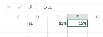
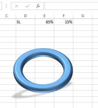
Let’s say we have to create the 3D doughnut KPI chart to Service Level metric.
- We are putting our Service level value on range “E1”
- Put formula “=1-E1” on range “F1”
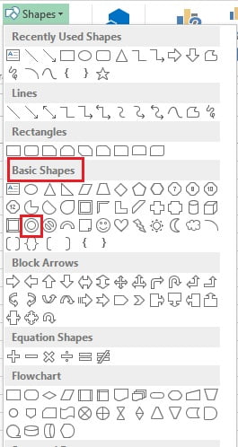
- Go to the Insert>>Shape>>Select the Doughnut available under Basic Shapes
- Drag the shape on the worksheet.
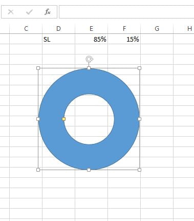
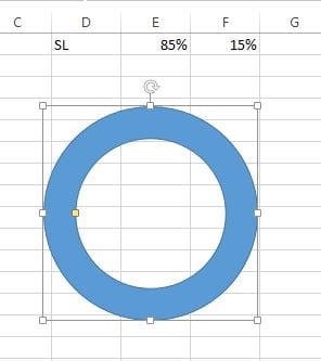
- Pick the yellow handle of the shape and change the width of Doughnut.
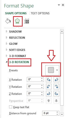
- Right click on the Doughnut and click on Format Shape.
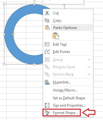
- In the Format Shape window select the Shape Effects.
- Go to 3-D Rotation option and select the preset.
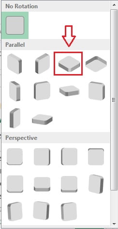
- Select the Isometric Top Up preset in the Parallel.
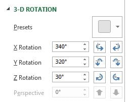
- Now change the X Rotation = 340°, Y Rotation = 320°, Z Rotation = 30°
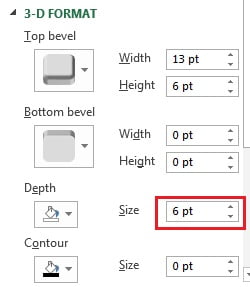
- Go to the 3-D Format option in Effects.
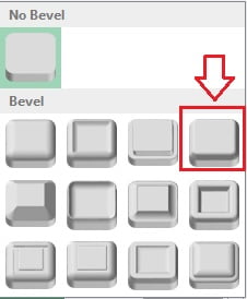
- Select the Top bevel.
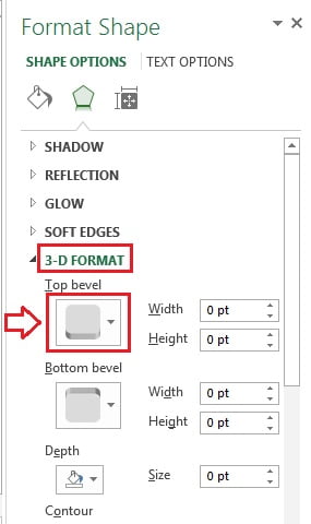
- Select the Cool Slant Bevel from the list.
- Change the Depth as 6pt in 3-D Format.
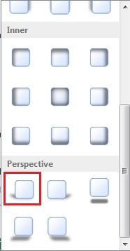
- Now go to Shadow under Effects option and select Preset.
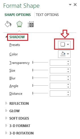
- Choose the Perspective Diagonal Upper Left shadow under Perspective.
- Our Doughnut shape is ready to use. It will look like below image.
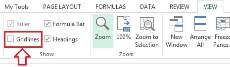
- Now remove the gridlines from the worksheet.
- Click anywhere on the worksheet.
- Go to View tab and uncheck the Gridlines checkbox.
- Select the range “E1:F1”
- Go to Insert>>Charts>>Insert 2D Pie Chart.
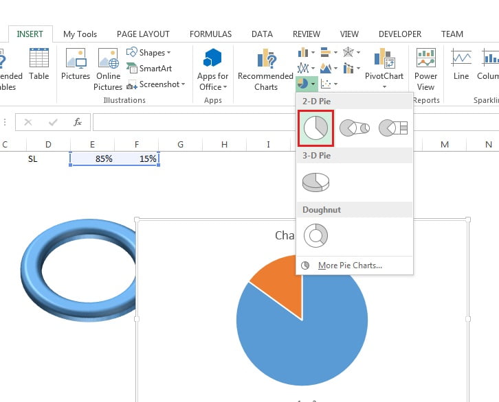
Insert Pie Chart
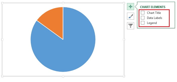
- Remove all the elements from the Chart like – Title and Legend
- Keep the chart over the Doughnut Shape.
- Now Select the Chart Area and go the format Tab.
- Take the Shape as No Fill.
- Take the Outline as No Outline.
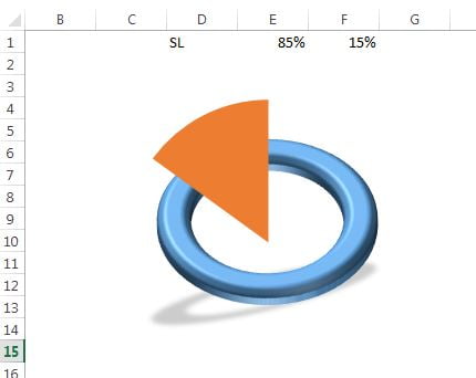
- Double click on blue Slice in the Pie chart. It will be selected.
- Right click and click on Format Data Series.
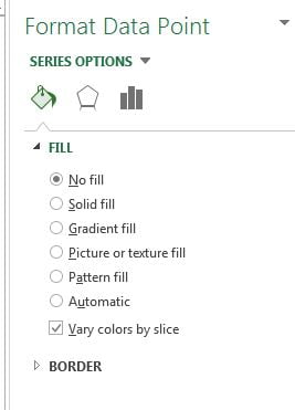
- Go to Fill and Line option and Fill as No fill
- Border as No Line.
- After doing the above given formatting our chart will look like below image.
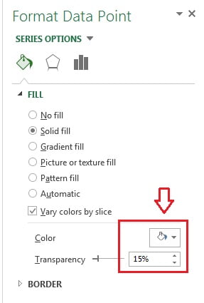
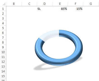
- Double click on the Orange Slice of Pie chart. It will be selected.
- Fill the Color as White color.
- Give the Transparency as 15%.
- After doing the above given settings our chart will look like below image.
- Now we will add the Data Labels.
- Go to the Insert tab and select the Text Box.
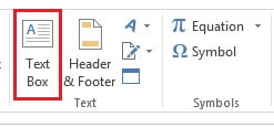
- Drag the Text Box on the worksheet.
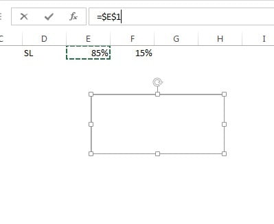
- Select the Text Box and go to Formula bar.
- Press “=” in formula bar and click on range “E1”
- Text Box value will be linked with the SL value.
- Select the Text box and go to Home tab.
- Change the Vertical and Horizontal alignment as Center.
- Take the Font Name as “Impact“
- Take the Font Size as “35“
- Put the Text box in the center of Doughnut.
Our 3D Doughnut Chart is ready and It will look like below image.

Click to buy 3D Doughnut Chart for KPI Metrics
Visit our YouTube channel to learn step-by-step video tutorials
Video Tutorial for 3D Doughnut Chart for KPI Metrics
Click to buy 3D Doughnut Chart for KPI Metrics