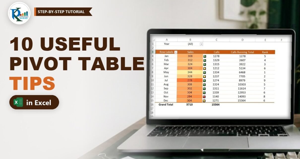
These 10 pivot table tips fix the small annoyances that slow down every Excel report: column widths that jump on refresh, running totals and ranks you still build with helper formulas, and copying the same report onto a sheet for every year. Each tip takes less than a minute, and every one is demonstrated in the free practice workbook, which has a separate sheet for each tip. They work in Excel 2013, 2016, 2019, 2021 and Microsoft 365 on Windows.
⬇️ Download the Practice File
11 sheets (one per tip plus Data) · .xlsx (no macros) · Excel 2013 and later
Watch the Video Tutorial
The video walks through the practice file sheet by sheet, from fixing the column width to repeating item labels, and ends with a bonus example built for a viewer.
What These Pivot Table Tips Cover
- Keep your layout – stop column widths and formatting from resetting on every refresh.
- Calculate inside the pivot – running totals and ranks with Show Values As, no helper columns.
- Move and multiply reports – move a pivot anywhere and create one sheet per year in a single click.
- Share and highlight – put a live pivot in PowerPoint or Word and apply conditional formatting that ignores the Grand Total.
- Clean, flat layouts – filter by selection, tabular form and repeated labels.
The Practice Data
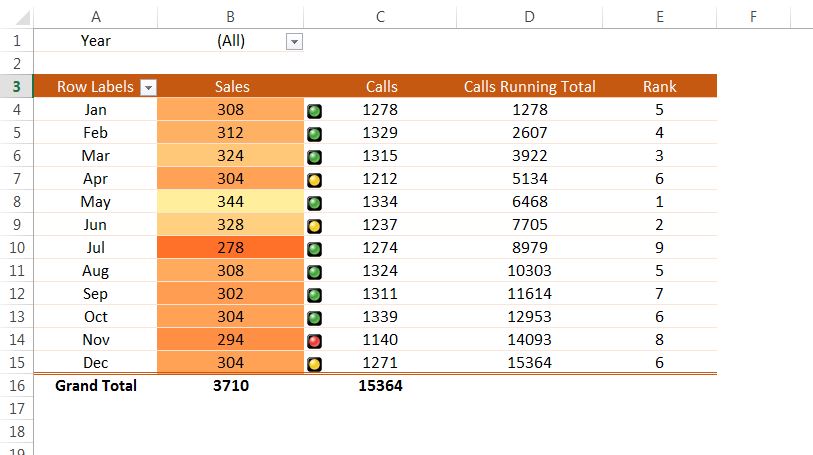
The Data sheet holds 60 rows (A1:D61) with four columns: Year (2015 to 2019), Month, Sales and Calls. Most tip sheets use the same layout: Year in the Filters area (cell B1 shows (All)), Month in Rows and Sum of Sales in Values. For all five years together, the grand total is 3,710 sales and 15,364 calls.
Part 1 – Keep the Pivot Table Layout Stable
Tip 1: Fix the column width
You widen a column to fit a long heading, press Refresh, and Excel shrinks it again. To stop that:
- Set the column widths you want.
- Right-click any cell in the pivot table and choose PivotTable Options (or Analyze > Options; in Microsoft 365 the tab is called PivotTable Analyze).
- On the Layout & Format tab, untick Autofit column widths on update and click OK.
Refresh now and the widths stay put. On the Fix Column Width sheet this option is already off, which is why column A stays wide after a refresh.
In the same dialog you will see Preserve cell formatting on update. It is ticked by default. If someone unticks it, any manual formatting you add to the pivot (a header colour, alignment, a bigger font) disappears on the next refresh. Make sure it is ticked when you want your formatting to survive.
Part 2 – Calculations with Show Values As
Tip 2: Add a running total
A running total shows the cumulative value: January shows January’s calls, February shows January plus February, and so on. On a normal sheet you would write a formula such as =SUM($C$4:C4) and fill it down, locking the first cell with F4 so the range grows row by row. Inside a pivot table you don’t need it:
- Open the field list (right-click > Show Field List) and drag Calls into Values a second time. You now have two Sum of Calls columns.
- Right-click a number in the second one and choose Show Values As > Running Total In.
- Pick Month as the base field (it is the row field) and click OK.
- Rename the header to Running Total.
In the practice file the column reads 1,278 for January, 2,607 for February, 3,922 for March, and finishes at 15,364 in December, which matches the Calls grand total.
Tip 3: Rank the months
To rank months by sales, add Sales to Values a second time and rename it Rank. Right-click it, choose Show Values As > Rank Largest to Smallest, pick Month as the base field and click OK. May, with the highest sales (344), becomes rank 1.
How pivot ranking differs from RANK
In the video PK first builds the same ranking with a worksheet formula, =RANK(C4,$C$4:$C$15,0), where 0 means descending. Compare the two results for July, the weakest month:
- The RANK formula gives July rank 12. Tied values share a rank and the next rank is skipped.
- The pivot rank gives July rank 9. In the practice file January and August both have 308 and share rank 5, while April, October and December (304 each) share rank 6. The pivot does not skip numbers after a tie.
Part 3 – Move and Multiply Your Pivot Table Reports
Tip 4: Move a pivot table
Click inside the pivot, go to Analyze > Actions > Move PivotTable and choose:
- Existing Worksheet – click the new top-left cell, on this sheet or any other sheet, and click OK.
- New Worksheet – Excel adds a sheet and places the pivot there, starting in column A.
Tip 5: Show Report Filter Pages (one sheet per year)
Need the same report for each year on its own sheet? Don’t copy the sheet five times and change the filter by hand.
- Put the field you want to split by (here Year) in the Filters area.
- Click the pivot, go to Analyze, open the Options drop-down in the PivotTable group and choose Show Report Filter Pages.
- Select Year and click OK.
Excel creates sheets named 2015, 2016, 2017, 2018 and 2019, each with a copy of the pivot already filtered to that year. Your original pivot stays where it was.
Tip 6: Put a live pivot table in PowerPoint or Word
A normal paste gives you a static table. To keep it editable:
- Copy the pivot table in Excel.
- In PowerPoint go to Home > Paste > Paste Special, select Microsoft Excel Worksheet Object and click OK.
- Resize the object as needed. To change it, double-click it: Excel’s ribbon opens inside the slide, so you can, for example, set the Year filter to 2015 and click outside to return.
The same Paste Special steps work in Microsoft Word.
Part 4 – Formatting and Filtering
Tip 7: Conditional formatting that skips the Grand Total
Select the Sum of Sales values, go to Home > Conditional Formatting > New Rule. Above the rule types, pivot tables give you three Apply Rule To options:
- Selected cells – only the cells you selected. If the pivot grows, new rows are not formatted.
- All cells showing “Sum of Sales” values – every Sum of Sales cell, including the Grand Total.
- All cells showing “Sum of Sales” values for “Month” – every month, but not the Grand Total.
The third option is usually what you want. Otherwise the Grand Total (3,710) takes the top colour and flattens the scale for every month. The practice file uses a 2-Color Scale from orange (lowest) to light yellow (highest) with the third option. To switch between options later, select the range, press Alt+O+D to open the Rules Manager and edit the rule.
Tip 8: Filter by selection
Select the row labels you want, right-click and choose Filter > Keep Only Selected Items. To do the opposite, choose Filter > Hide Selected Items. On the Filter Selected Item sheet only July to December are kept, so the Grand Total drops to 1,790.
Part 5 – Flat Layouts for Export
Tip 9: Tabular form
By default a pivot uses Compact Form, which stacks Year and Month in a single Row Labels column. Go to Design > Report Layout > Show in Tabular Form to give each row field its own column with a real header (Year, Month). It is easier to read and to copy elsewhere.
Tip 10: Repeat item labels
In tabular form the year appears only once, at the top of its group. To fill it down on every row, go to Design > Report Layout > Repeat All Item Labels. To finish a clean flat table:
- Right-click a year and untick Subtotal “Year” to remove the year subtotal rows.
- Go to Analyze and click +/- Buttons to hide the expand and collapse icons.
Compare the last two sheets: Tabular format still has its year subtotals (it ends in row 69), while Repeat Labels has repeated years and no subtotals (it ends in row 64).
Common Errors and Fixes
I can’t find the Analyze tab
The pivot tabs only appear when a cell inside the pivot is selected. In Excel 2013 they are called Analyze and Design; in Microsoft 365 they are PivotTable Analyze and Design. The commands are the same.
Show Report Filter Pages is greyed out
It needs at least one field in the Filters area. Drag Year (or any field) there first.
My formatting disappears after a refresh
Open PivotTable Options and tick Preserve cell formatting on update. For colour rules, use conditional formatting with the “for Month” option (Tip 7), which follows the pivot as it changes.
Tips
- Rename value headers (Running Total, Rank) so readers know a column is calculated.
- Use Report Filter Pages with any filter field, such as region or salesperson, not just years.
- Microsoft’s guide to Show Values As calculations in PivotTables lists every option, including % of total and difference from.
Want It Ready-Made?
If you want a polished pivot-based report rather than building one, the Stylish Pivot Chart with Slicer in Excel template on NextGenTemplates.com is a good starting point, or browse all Excel templates. To learn pivot tables, slicers and dashboards step by step, join the video course Excel Pivot Tables and Dashboards.
Related Tutorials
- Pivot Table Super Tips in Excel
- Conditional Formatting in a Pivot Table with 3 Examples
- Create Multiple Pivot Sheets in Seconds with Report Filter Pages
- Show Change % in a Pivot Table
- GROUPBY and PIVOTBY Functions in Excel
Frequently Asked Questions
How do I stop a pivot table from changing column width on refresh?
Right-click the pivot, open PivotTable Options and untick Autofit column widths on update on the Layout and Format tab. Set your widths first; they will stay after every refresh.
How do I add a running total in a pivot table?
Add the value field a second time, right-click it and choose Show Values As, then Running Total In, with the row field (Month in the practice file) as the base field.
Why does the pivot table rank differ from the RANK function?
Both give tied values the same rank, but RANK skips the following numbers while the pivot rank does not. In the example, July is rank 12 with RANK and rank 9 in the pivot.
How do I create a separate sheet for each filter value?
Put the field in the Filters area, then use Analyze, Options drop-down, Show Report Filter Pages. Excel creates one filtered copy of the pivot per item, each on a sheet named after that item.
Can I paste a pivot table into PowerPoint and still edit it?
Yes. Use Paste Special and choose Microsoft Excel Worksheet Object. Double-click the object in the slide to change filters or layout with the Excel ribbon.
How do I apply conditional formatting without the Grand Total?
In the New Formatting Rule dialog choose the third Apply Rule To option, all cells showing the value field for the row field. The rule then covers every month but skips the Grand Total.
About the Author
PK is a Microsoft Excel expert and trainer and the founder of PK: An Excel Expert and NextGenTemplates.com. He has been teaching Excel, Power Query and Power BI since 2016 on his YouTube channel.
Conclusion
These pivot table tips take seconds to apply and save time on every report: fix the column width, let Show Values As do running totals and ranks, move and split reports with built-in commands, keep a live pivot in PowerPoint, format only the months, and flatten the layout with tabular form and repeated labels. Download the practice file, open each sheet and try the tip on the same data before using it on your own reports.