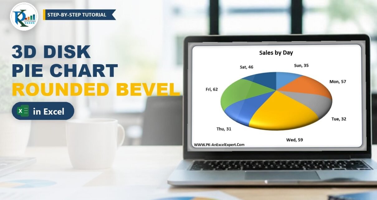
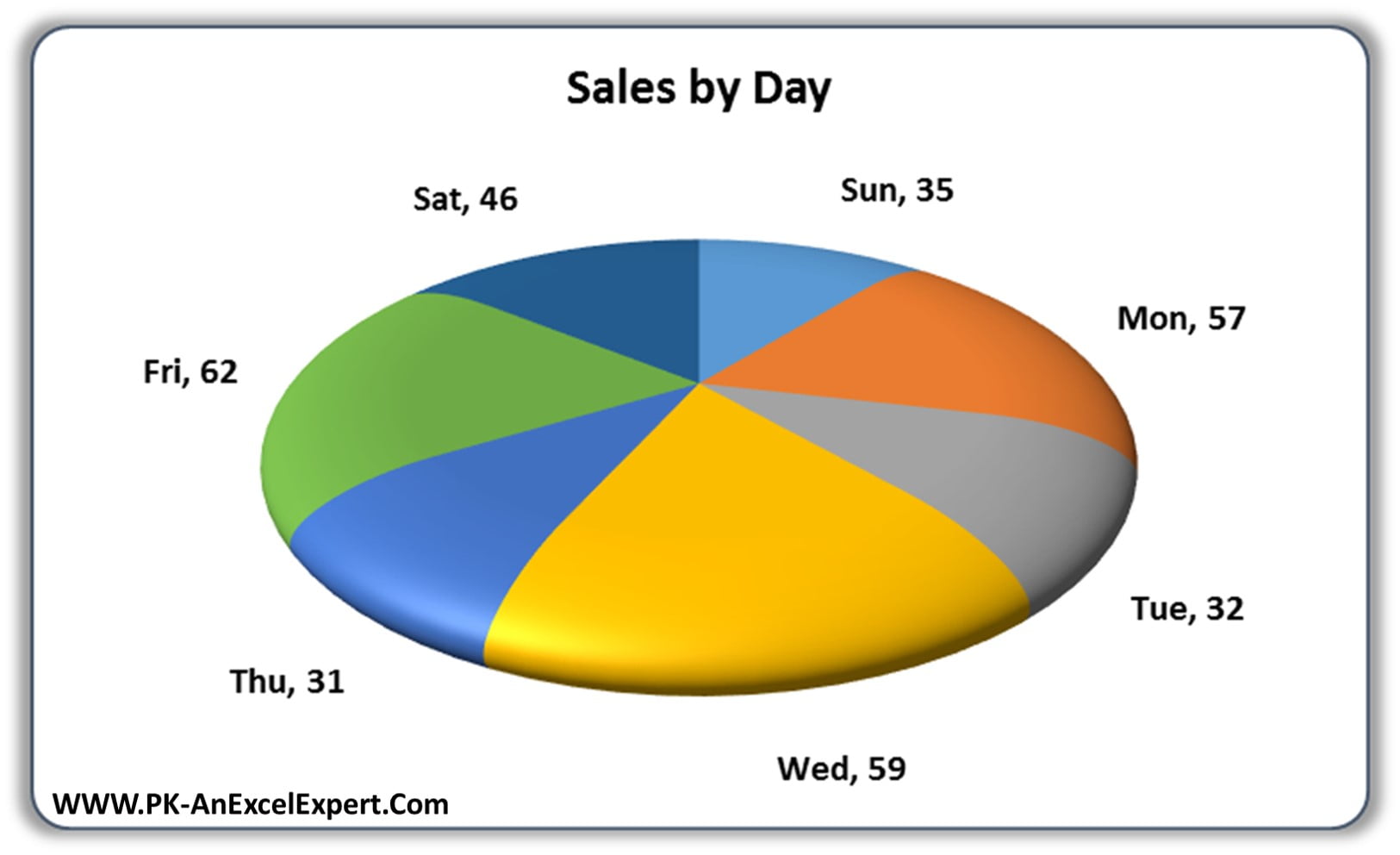
A 3D disk pie chart in Excel is a normal 3-D pie with one formatting trick: a large rounded bevel on the top and bottom of the series. That bevel turns the flat, sharp-edged pie into a smooth, rounded disk that looks like a polished button. It takes about two minutes, needs no add-ins and no VBA, and works with any data you would put in a pie chart. In this tutorial you will build the exact chart from PK’s video, using day-wise sales, and you can download the finished file to compare your settings.
⬇️ Download the 3D Disk Pie Chart
Two-sheet workbook · .xlsx (no macros) · Excel 2010 and later
Watch the Video Tutorial
In the video PK copies the sales table to a new sheet, inserts a 3-D pie, sets a Circle bevel of 100 pt on the top and bottom, and finishes with category-name labels placed outside the slices.
What You Will Build
- A 3-D pie chart of sales by weekday (Sun to Sat) from a simple two-column table.
- A rounded disk effect made with a Circle bevel of 100 pt width and 100 pt height on both the top and the bottom.
- Clean slice separators from thin white borders between the slices.
- Readable data labels that show the day and the value, for example Fri, 62, at the Outside End position.
- A presentation-ready chart with a bold title and no legend, ready for a dashboard or a slide.
The Sample Data
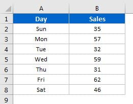
The workbook uses a small table in A1:B8: the header Day in A1, Sales in B1, and one row per weekday underneath.
| Day | Sales |
|---|---|
| Sun | 35 |
| Mon | 57 |
| Tue | 32 |
| Wed | 59 |
| Thu | 31 |
| Fri | 62 |
| Sat | 46 |
The seven values add up to 322. A pie chart shows each value as a share of that total, so Friday (62) gets the biggest slice and Thursday (31) the smallest. You can type this table or use your own categories; the steps are the same.
Part 1 – Insert the 3-D Pie Chart
Step 1: Prepare the sheet
In the video PK pastes the table on a fresh sheet and switches off gridlines from View › Gridlines, so the finished chart sits on a clean white background. He also gives the table a quick header style. Any formatting is fine; it does not change the chart.
Step 2: Insert a 3-D Pie
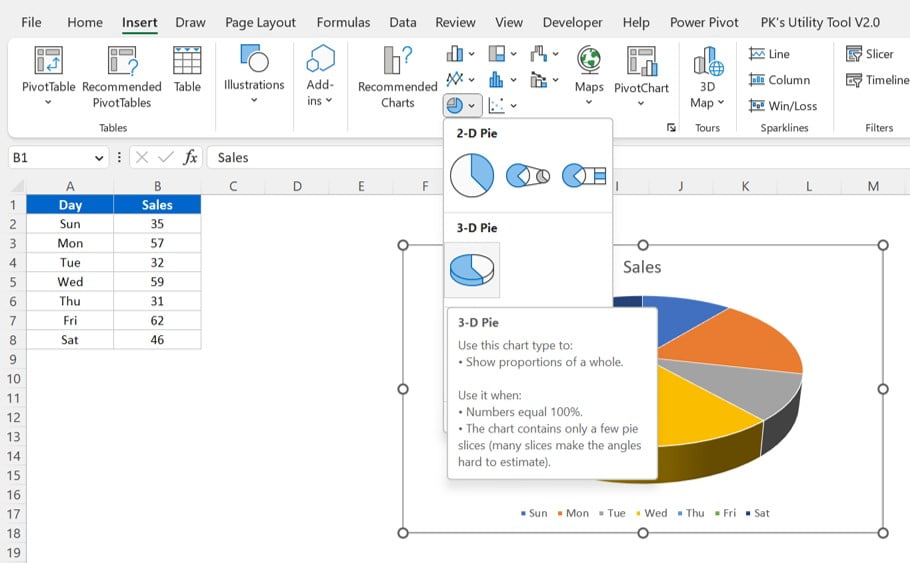
Select A1:B8 and go to Insert › Insert Pie or Doughnut Chart › 3-D Pie. Because the header row is included, Excel names the series Sales and uses the days as categories.
Step 3: Tidy the title and legend
Click the legend and press Delete; the labels you add later will name each slice, so the legend is not needed. Click the chart title and type Sales by Day, then make it black and bold from the Home tab. The sample file uses a 14 pt bold title.
Part 2 – Turn the Pie into a 3D Disk
This is the part that creates the disk look. Everything happens in the 3-D Format settings of the data series.
Step 4: Open Format Data Series
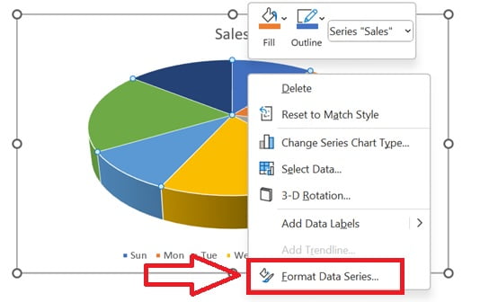
Right-click any slice once (so the whole series is selected, not one slice) and choose Format Data Series.
Step 5: Go to Effects › 3-D Format
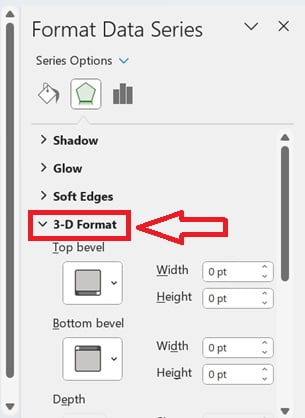
In the pane, click the Effects icon (the pentagon) and expand 3-D Format. You will see Top bevel and Bottom bevel, both at 0 pt by default.
Step 6: Choose the Circle bevel for top and bottom
Open the Top bevel gallery and pick Circle (the first preset). Do the same for Bottom bevel. Setting both matters: the top bevel rounds the upper face and the bottom bevel rounds the underside, so the edge looks curved all the way round instead of only from above.
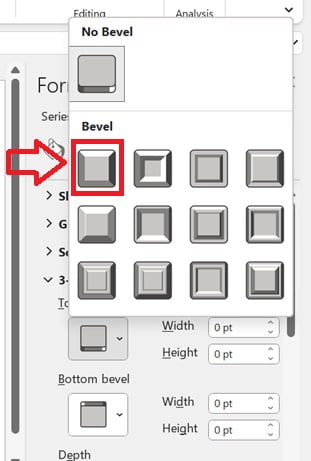
Step 7: Set width and height to 100 pt
Type 100 pt in all four boxes: Top bevel Width and Height, and Bottom bevel Width and Height. The pie immediately turns into a smooth disk.
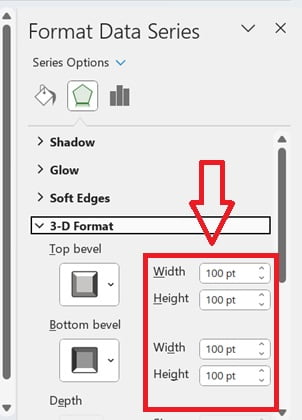
Why the bevel creates the disk
- A bevel rounds the edges of a 3-D shape. Width controls how far the rounding reaches in from the edge, and Height controls how tall the rounded part is.
- With a small value, say 6 pt, only a thin rim is rounded and the pie still looks like a cut cake.
- At 100 pt the rounding covers most of each slice, so the top surface becomes one smooth curve and the slices together read as a single domed disk.
- Using the same value on top and bottom keeps the shape symmetric, like a coin or a button.
The sample workbook also has a 2 pt white border around each slice (Format Data Series › Fill & Line › Border, white solid line). That thin white line is what separates the coloured slices so cleanly on the rounded surface.
Part 3 – Add and Format the Data Labels
Step 8: Add data labels
Right-click the chart and choose Add Data Labels, or use the Chart Elements (+) button next to the chart and tick Data Labels. At this point each slice shows only its value.
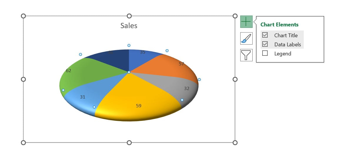
Step 9: Show the category name
Right-click any label and choose Format Data Labels. Under Label Contains, tick Category Name and leave Value ticked. Keep Show Leader Lines on. The default separator is a comma, which gives labels such as Mon, 57.
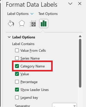
Step 10: Put the labels outside
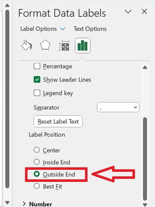
Still in Label Options, set Label Position to Outside End. The labels move off the curved surface, where they are easy to read. Finally make the label font black and bold and a little bigger from the Home tab (the sample uses 10 pt bold).
That is the complete chart. On the first sheet of the download the chart area also has rounded corners and a soft outer shadow (Format Chart Area › Border › Rounded corners, and Effects › Shadow), which gives the card look you see in the hero image.
Common Errors and Fixes
Only one slice turned into a disk
You clicked a slice twice, which selects that single data point. Click an empty part of the chart, then click the pie once so all slices are selected, and apply the bevel again.
The pie still has sharp edges
Check that both Width and Height are 100 pt for the top and the bottom bevel. If only the top bevel is set, the underside stays flat and the edge looks cut.
Labels show only numbers
Category Name is not ticked. Open Format Data Labels and tick it under Label Contains.
Labels overlap on small slices
This is an added tip, not from the video: drag an individual label a little further out (leader lines follow it), reduce the label font size, or combine very small categories into an Other row before charting.
Tips for a Better 3D Disk Pie Chart
These tips are general Excel advice added to PK’s method:
- Keep it to about six or seven slices. A pie with many thin slices is hard to read, disk or not.
- Use the same bevel recipe on a doughnut chart or a single-value KPI pie to get a matching rounded look across a dashboard.
- Try other bevel presets such as Soft Round or Convex for a different finish, and compare them against Circle.
- Avoid using a disk pie for precise comparisons; when the values are close, a bar chart is easier to judge.
- Microsoft’s guide on how to add a pie chart covers the basic pie options in every Excel version.
Want It Ready-Made?
If you would rather start from finished, polished charts, the Data Analyst’s Chart & Visualization Pack on NextGenTemplates.com bundles 10 premium Excel and Google Sheets chart templates, or you can browse all Excel chart templates. To learn charts, infographics and dashboards step by step, join the video course Excel Pivot Tables and Dashboards on the NextGenTemplates Academy.
Related Tutorials
- Pie Chart in Excel: Insert, Label and Explode Slices
- Pie of Pie Chart in Excel
- Chart Elements in Excel: Titles, Labels, Legend and Axes
- 3D Doughnut Chart for KPI Metrics
- Analog Clock in Excel with a Pie and Doughnut Chart
Frequently Asked Questions
What is a 3D disk pie chart in Excel?
It is a standard 3-D pie chart with a large Circle bevel on the top and bottom of the data series. The bevel rounds the slices so the pie looks like a smooth disk instead of a flat cut cake.
Which bevel settings make the disk effect?
In Format Data Series, open Effects and then 3-D Format. Choose the Circle bevel for both Top bevel and Bottom bevel, and set Width and Height to 100 pt in all four boxes.
Can I use a 2-D pie instead of a 3-D pie?
The video and the sample file both start from the 3-D Pie chart type, which gives the tilted view that shows off the rounded edge. Start from 3-D Pie to get the same result.
How do I show the day name and value on each slice?
Add data labels, open Format Data Labels, tick Category Name together with Value, and set the Label Position to Outside End.
Do I need VBA or an add-in to make this chart?
No. The chart uses only built-in chart formatting. The download is a normal .xlsx file with no macros.
About the Author
PK is a Microsoft Excel expert and trainer and the founder of PK: An Excel Expert and NextGenTemplates.com. He has been teaching Excel, Power Query and Power BI since 2016 on his YouTube channel.
Conclusion
A 3D disk pie chart in Excel is one of the quickest ways to make a plain pie look professional. Insert a 3-D pie, give the series a Circle bevel of 100 pt on the top and bottom, add category-name labels at Outside End, and remove the legend. Download the sample file, compare your settings with PK’s chart, and reuse the same bevel recipe in your next dashboard or presentation.