Multiple KPIs Visualization in Excel with Dynamic RAG Colors

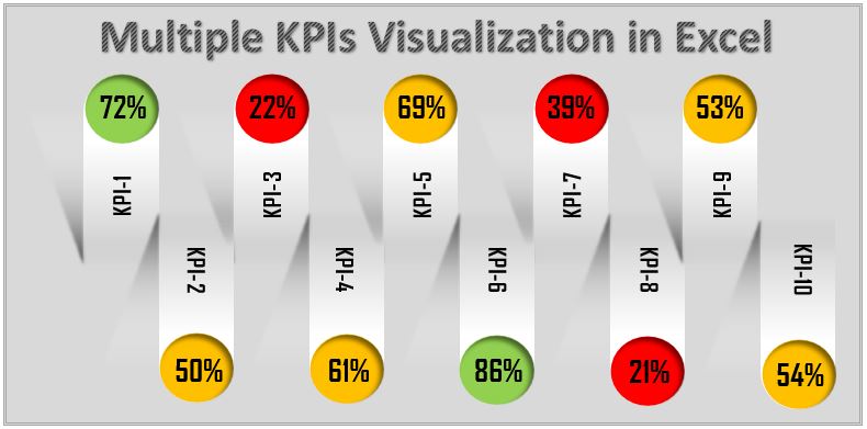
A multiple KPIs visualization in Excel lets you show ten KPIs in one eye-catching panel, with each result in a circle that turns red, amber or green on its own. In this tutorial you build it from scratch with ordinary Excel shapes: glossy pillars made with gradient fills, three colored circles, a linked picture driven by named ranges, and text boxes that read the numbers from the sheet. Change a KPI value and its circle switches color instantly, so you can drop the panel straight into a KPI dashboard or a business presentation.

Watch the Video Tutorial

PK builds the whole visual in a new workbook: the color code formula, the gradient pillars, the RAG circles on a support sheet, the linked picture with INDIRECT names and the linked labels.

What You Will Build

• A color code column that labels each KPI Red, Amber or Green with one IF formula.
• Ten glossy pillars made from a rounded rectangle and a shaded triangle, flipped top and bottom.
• Dynamic RAG circles: one linked picture per KPI that shows the correct colored circle.
• Linked labels for the performance value and the KPI name, so the visual always matches the data.
• A layout that works for percentages, numbers or decimals.

Step 1: Prepare the KPI Data and the Color Code

Enter the KPI data

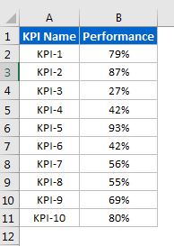
Put the KPI names in A1:A11 (header KPI Name, then KPI-1 to KPI-10) and the results in B1:B11 (header Performance). In the video PK fills the Performance column with RANDBETWEEN so that every recalculation (F9) shows new values and new colors. In a real file, type or link your actual KPI results.

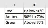
Decide the RAG rules

The tutorial uses these thresholds:

Add the color code formula

Type Color code in C1 and enter this in C2, then fill it down to C11:

=IF(B2<50%,"Red",IF(AND(B2>=50%,B2<=70%),"Amber","Green"))

Below 50% returns Red. Between 50% and 70% (both included) returns Amber. Anything else returns Green. The exact words matter, because in Step 5 they become the names of three cells. If one KPI needs different limits, give that row its own IF; the rest of the build does not change.

Finally go to View and untick Gridlines so the visual sits on a clean sheet.

Step 2: Draw the Background Panel

Select a block of empty cells to the right of the data, large enough for ten pillars. On the Home tab give it a light grey fill. Then right-click, choose Format Cells → Border, pick a darker grey, choose a line style and click Outline. This grey box is the canvas for everything that follows.

Step 3: Build the Glossy Pillars

The pillar

1. Go to Insert → Shapes and insert a rounded rectangle. Make it tall and narrow.
2. Drag the yellow handle to change the corner radius until the top looks like an arch.
3. Set Shape Outline → No Outline.
4. Right-click → Format Shape → Fill & Line → Gradient fill. Keep a linear gradient with a 90° angle and delete one of the default stops.
5. Set the first stop to white at about 35-40% position, the second stop to grey at about 80%, and the last stop to the same grey with 100% transparency.

The pillar is now white at the top and fades into the background at the bottom.

The shadow

1. Insert a right triangle and rotate it 180°: Format → Rotate → Rotate Right 90° twice.
2. Resize it and place it along the side of the pillar. Set No Outline.
3. In Format Shape, use a gradient with only two stops: white and black. Choose a direction that runs across the triangle, then set the white stop to 100% transparency.
4. Add Shape Effects → Soft Edges → 2.5 pt to blur it.
5. Right-click the triangle and choose Send to Back.

Select the pillar and the triangle, right-click and choose Group.

Make ten pillars

Copy the group, then use Format → Rotate → Flip Vertical on the copy so it hangs from the bottom. Place it next to the first one and group the pair. Copy the pair until you have five pairs, which gives ten pillars. Select them all and use Align → Align Top and Align → Distribute Horizontally so the spacing is even.

Step 4: Create the RAG Circles on a Support Sheet

1. Insert an Oval and hold Shift while you size it so it stays a perfect circle.
2. Remove the outline, fill it green and add Shape Effects → Shadow with an inner shadow for depth.
3. Add a new sheet and name it Support. Paste the circle there.
4. Right-click the circle → Size and Properties → Properties and choose Don’t move or size with cells.
5. Resize column A and row 1 so the circle fits inside cell A1.
6. Paste two more circles into B1 and C1. Copy A1 and use Paste Special → Column widths on B1:C1 so all three cells are the same size.
7. Recolor the circle in B1 amber and the circle in C1 red, and turn off the gridlines on this sheet too.

Each cell now holds exactly one colored circle: green in A1, amber in B1 and red in C1.

Step 5: Make the Circles Dynamic with a Linked Picture

Paste a linked picture

Copy any one of the three cells on the Support sheet. Go back to the KPI sheet and choose Home → Paste → Paste Special → Linked Picture. You now have a live picture of that cell, circle included.

Name the three color cells

Go to Formulas → Name Manager → New and create three names on the Support sheet:

• Green refers to =Support!$A$1
• Amber refers to =Support!$B$1
• Red refers to =Support!$C$1

Create one name per KPI

Now add ten more names. Names cannot contain spaces, so use an underscore:

KPI_1   =INDIRECT(Sheet1!$C$2)
KPI_2   =INDIRECT(Sheet1!$C$3)
...
KPI_10  =INDIRECT(Sheet1!$C$11)

Point each picture at its KPI

Select the linked picture, click in the formula bar, type =KPI_1 and press Enter. Press Ctrl+D to duplicate the picture, place one copy on each pillar end, and change the formula of each copy to =KPI_2, =KPI_3 and so on up to =KPI_10.

How the dynamic circle works

• C2 holds a word such as Amber, produced by the IF formula.
• INDIRECT(Sheet1!$C$2) turns that word into a reference. Because Amber is also a defined name, INDIRECT returns the cell Support!B1.
• The linked picture shows whatever cell its name returns, so it shows the amber circle.
• When the performance changes, C2 changes to Red or Green, INDIRECT points to a different cell and the picture swaps circles instantly.

Step 6: Add the Linked Labels

Performance value

1. Insert a Text Box, select it, click in the formula bar, type =, click B2 and press Enter. The box now shows the KPI-1 value and follows it.
2. Set Shape Fill: No Fill and Shape Outline: No Outline, make the font larger and bold, centre it and pick a condensed font (PK uses Agency FB).
3. Duplicate it onto every circle and relink each copy to its own cell: B3, B4 and so on.

Relinking can reset the formatting. Select the first, finished text box, double-click the Format Painter on the Home tab and click each of the other boxes to copy the look in one go. Press Esc when you are done.

KPI name

Copy a text box once more and link it to the KPI name in A2. Rotate it 90° so a longer name fits along the pillar, make it bold, then duplicate it for every pillar and link each copy to A3, A4 and so on. Use the Format Painter again to match them. Your multiple KPIs visualization is ready.

Modern Excel Alternative

This section is an addition from general Excel practice; it is not part of the video.

In Excel 2019 and Microsoft 365 the color code can be written with IFS, which is easier to read when you have several bands:

=IFS(B2<50%,"Red",B2<=70%,"Amber",TRUE,"Green")

IFS stops at the first true test, so the Amber test only needs the upper limit. For KPIs measured as numbers, replace 50% and 70% with your own limits, or put the limits in cells and refer to them so you can change the rules without editing formulas.

Common Errors and Fixes

This section and the Tips below are additions from general Excel practice; they are not shown in the video.

A circle goes blank or does not change color

The word in the color code column does not match a defined name exactly. Check for extra spaces and spelling: Red, Amber and Green in the IF formula must match the three names in Name Manager.

The circles shift or get squashed

The circles on the Support sheet are still set to move and size with cells. Set each one to Don’t move or size with cells, and keep A1:C1 the same width and height.

Excel will not accept the name

Names cannot contain spaces or start with a number, and they must not look like a cell address. KPI_1 works; KPI 1 and KPI1 do not (KPI1 is a valid cell reference in modern Excel).

Tips

• Keep the RAG limits in cells next to the data, so managers can adjust targets without touching formulas.
• Group all pillars, pictures and labels when you are finished so the visual moves as one object.
• Microsoft documents the function used for the dynamic names in INDIRECT function.

Want It Ready-Made?

If you would rather start from the finished file, the Multiple KPIs Visualization in Excel template is available on NextGenTemplates.com, and you can browse more Excel charts and visualization templates. To learn charts, infographics and dashboards step by step, join the video course Excel Pivot Tables & Dashboards: Basic to Advanced on NextGenTemplates Academy.

Related Tutorials

• RAG (Red, Amber and Green) Analysis Chart in Excel
• One-Pager KPI Dashboard in Excel
• Candle Infographic Chart in Excel
• Sales Funnel Infographic Chart in Excel
• Convert Your Boring Bar Chart into Stylish Charts

Frequently Asked Questions

How do I show RAG status for many KPIs in Excel?

Give each KPI a color code with an IF formula, keep one red, one amber and one green circle in three named cells, and show the right one with a linked picture whose formula uses INDIRECT on the color code.

Why does the tutorial use INDIRECT?

INDIRECT converts the text in the color code cell into a reference. Because Red, Amber and Green are defined names, the text becomes the cell that holds that circle.

Can I use numbers instead of percentages?

Yes. Only the IF formula changes. Replace the percentage limits with the number limits for each KPI and the circles and labels work the same way.

Does this need VBA or a chart?

No. It uses shapes, a linked picture, defined names and one formula per KPI, so it works in any desktop version of Excel that supports linked pictures.

Can I add more than ten KPIs?

Yes. Add rows to the data, copy another pillar pair, and create a new KPI name and linked picture for each extra row.

About the Author

PK is a Microsoft Excel expert and trainer and the founder of PK: An Excel Expert and NextGenTemplates.com. He has been teaching Excel, Power Query and Power BI since 2016 on his YouTube channel.

Conclusion

This multiple KPIs visualization in Excel looks like a designed infographic, yet it is built from a single IF formula, a few gradient shapes, three colored circles and a linked picture driven by INDIRECT names. Once the pieces are in place, every circle and label updates by itself when your KPI results change. Build it once, group it, and reuse it in every dashboard and presentation that needs a clear RAG view.