This sales dashboard in Excel 2013 Power View is a legacy example: it shows how PK built an interactive report with cards, a pie chart, a bar chart, a line chart and a clickable map using Power View, the visual report sheet that shipped with Excel 2013. Power View has since been removed from current Excel, so treat this page as a record of how the dashboard was made in 2019 and as a guide to rebuilding the same layout today. You will see the original steps from the video, then two modern alternatives: PivotCharts with slicers in Excel, and Power BI Desktop.
Version and compatibility note
Power View is no longer part of current Excel. Microsoft removed it from Excel for Microsoft 365 starting in October 2021 (Silverlight, which it relied on, reached end of support on October 12, 2021), and Excel 2021 and later do not include it. Older perpetual versions such as Excel 2016 and 2019 may still contain it, but it might have to be turned on before it appears, and Excel 2013 itself reached end of support on April 11, 2023. In Excel 2013, Power View needed Microsoft Silverlight to run. The steps below describe the original Excel 2013 workflow; they are not expected to work in Microsoft 365.
Watch the Video Tutorial
In the video PK switches on the Power View add-in in Excel 2013, inserts a Power View sheet from a sales table and builds the cards, map, tiles, pie, bar and line charts one by one.
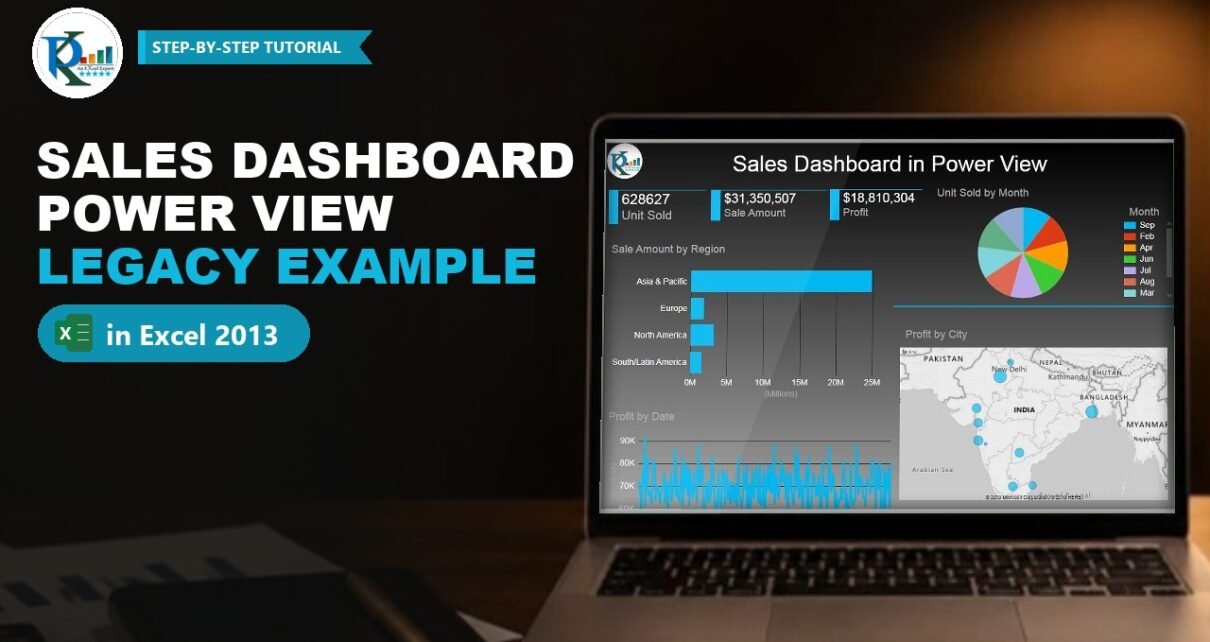
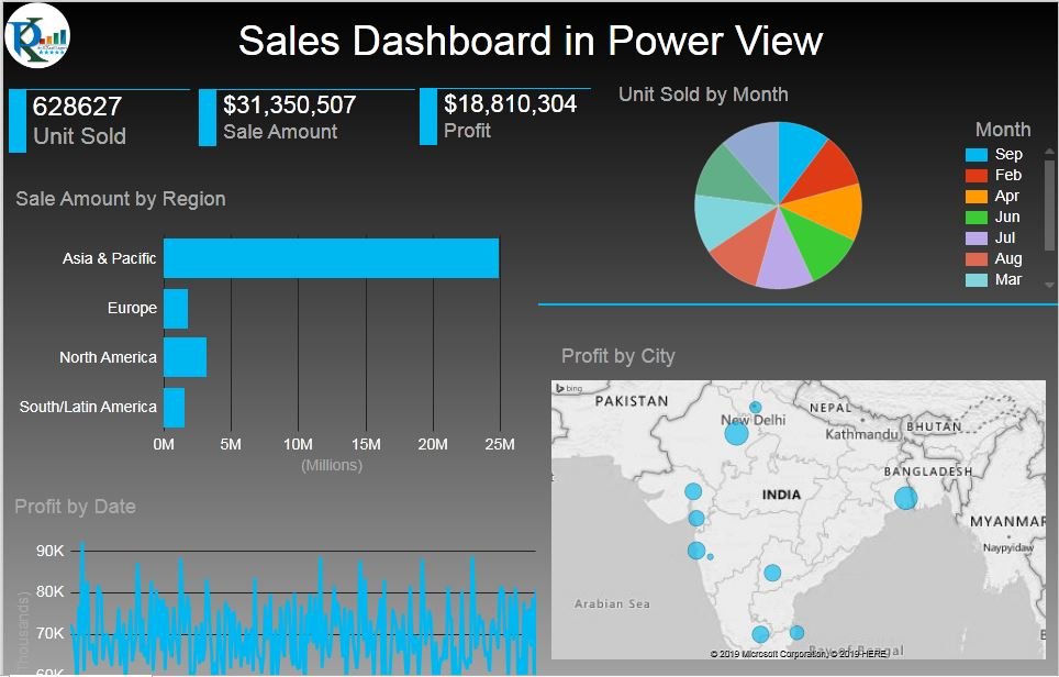
What the Legacy Dashboard Shows
- Three cards: Unit Sold, Sale Amount and Profit.
- Unit Sold by Month: a pie chart with a slice for each month.
- Sale Amount by Region: a bar chart for Asia & Pacific, Europe, North America and South/Latin America.
- Profit by Date: a line chart of daily profit.
- Profit by City: a map with bubbles per city, plus country tiles (India, Japan, Mexico, Singapore and more) that switch the map to another country.
- Cross-filtering: click a city, a month slice or a region bar and every other visual filters to it.
The Sales Data
All visuals come from one sheet, Sales Data, with daily rows starting on 1 January 2019. The columns are:
- Date and Month
- City, Country and Region (for example Jaipur, India, Asia & Pacific or London, United Kingdom, Europe)
- Unit Sold, Price per unit and Sale Amount
- Cost per Unit and Profit
PK recommends converting the range into an Excel table first (Insert → Table), so new rows are picked up automatically. That advice still applies to every modern alternative below.
How the Power View Sales Dashboard Was Built in Excel 2013
These steps come from the video and are kept as a historical reference.
Step 1: Enable the Power View add-in
On the Developer tab PK clicks COM Add-ins and ticks Power View. In the video Power Map is ticked too, because it had been downloaded separately for Excel 2013. If Excel asked to install Microsoft Silverlight at this point, Power View would not run until it was installed.
Step 2: Insert a Power View sheet
With a cell in the table selected, Insert → Power View opens the Insert Power View dialog. It offers Create a Power View sheet or Add selected data to an existing Power View sheet. A new sheet starts with a default table of a few columns, which PK deletes so he can build the layout from scratch, and then types the title Sales Dashboard at the top.
Step 3: Choose a theme and background
The Power View tab holds themes and backgrounds. The default background is white; PK picks a dark gradient so the blue visuals stand out.
Step 4: Create the three cards
From the Power View Fields list, drag Unit Sold onto the canvas. It appears as a small table; use the visual’s drop-down to switch it to a Card. Card Style offers a Callout look too, but PK keeps the plain card. Copy and paste the card twice, then replace the field with Sale Amount and Profit.
Step 5: Build the map and the country tiles
Drag Country and a value onto the canvas and click Design → Map to turn it into a Bing map. To get the final layout, move Country to TILE BY, put City in LOCATIONS and Profit in SIZE. Then choose Tile Type → Tile Flow so the country names run as a strip of tiles under the map. Clicking Japan, for example, redraws the map with the Japanese cities.
Step 6: Add the pie, bar and line charts
- Unit Sold by Month: drag Month and Unit Sold, then Other Chart → Pie.
- Sale Amount by Region: drag Region and Sale Amount, then Bar Chart → Clustered Bar.
- Profit by Date: drag Date and Profit, then Other Chart → Line.
Resize each visual to fit the grid shown in the screenshot.
Step 7: Add a logo and review
Use the picture option on the Power View tab to insert a company logo, then switch off Fit to Window to see the sheet at full size. Click a city bubble or a month slice to check that the cards and charts filter together.
Modern Alternative 1: PivotCharts with Slicers in Excel
This section is an addition and is not part of the original video. You can rebuild the same interactive layout in any current version of Excel with PivotTables, PivotCharts and slicers:
- Convert the Sales Data range into a table and insert a PivotTable on a new sheet for each view: Unit Sold by Month, Sale Amount by Region and Profit by Date.
- Insert a PivotChart from each PivotTable: a pie or doughnut for months, a bar chart for regions and a line chart for dates.
- For the three cards, use small PivotTables with only one value each, or link a text box to a cell that holds the total.
- Insert Slicers for Country, City and Region and a Timeline for Date. Right-click each slicer, choose Report Connections and tick every PivotTable so one click filters the whole page.
- For the map, use a Filled Map chart by country from a regular range, or show Profit by City as a sorted bar chart.
The main difference from Power View is that a PivotChart does not cross-filter other charts when you click it. Slicers and the timeline do that job instead.
Modern Alternative 2: Rebuild It in Power BI Desktop
This section is an addition and is not part of the original video. Power BI Desktop is the natural successor to Power View. Every visual in this dashboard has a direct match: Card, Pie chart, Clustered bar chart, Line chart and a map visual, with click-to-filter interactions between them by default.
- For a new report, use Get data → Excel workbook and load the Sales Data table.
- If you have an old workbook with a Power Pivot data model, Power BI Desktop offers File → Import → Power Query, Power Pivot, Power View. It converts queries, measures and relationships and shows a summary of anything it could not import. Check that summary rather than assuming every Power View sheet comes across unchanged.
- Add Country, City and Month slicers to replace the country tiles.
Common Problems and Fixes
There is no Power View button in my Excel
This is expected in Excel for Microsoft 365, Excel 2021 and later, where Power View has been removed. Use one of the two modern alternatives above.
Power View asks for Silverlight
Excel 2013 needed Microsoft Silverlight for Power View. Silverlight is no longer supported, so on a current machine the better path is a PivotChart or Power BI rebuild.
An old workbook opens but the Power View sheet is blank
The sheet was created by a component your Excel no longer has. The data sheet and any data model are still there, so you can rebuild the visuals from them.
Tips
- Keep your data in one clean table with a real Date column; it works in Power View, PivotTables and Power BI alike.
- Use the same three headline numbers (units, sales, profit) at the top of whichever tool you choose; readers look there first.
- Prefer a bar chart over a pie when you have more than five or six categories, such as twelve months.
- Keep one dark or one light theme across the page; PK’s dark background works because every visual uses the same blue.
- Microsoft’s guide to importing Excel workbooks into Power BI Desktop explains what converts and what does not.
Want It Ready-Made?
The original workbook is available as Sales Dashboard Power View in Excel 2013 on NextGenTemplates.com. It needs a version of Excel that still has Power View, so check your setup before buying. For a current tool, the Sales Dashboard in Power BI covers the same kind of analysis, and you can browse more Excel dashboard templates. To learn the PivotChart and slicer method properly, take the course Excel Pivot Tables and Dashboards on NextGenTemplates Academy.
Related Tutorials
- Stylish Pivot Chart with Slicer in Excel
- Connect Charts and Slicers in Excel in Seconds
- Create Relationship in Power Pivot
- Design, Publish and Share a Sales Dashboard in Power BI
- More Sales Dashboards in Excel
Frequently Asked Questions
Is Power View still available in Excel?
No. Microsoft removed Power View from Excel for Microsoft 365 starting in October 2021, and Excel 2021 and later do not include it. It only remains in older perpetual versions, which are themselves out of support.
What replaced Power View?
Power BI Desktop is the main replacement for interactive reports. Inside Excel, PivotCharts with slicers and timelines give you a similar click-to-filter dashboard.
Can I open an old Power View workbook in Power BI?
Power BI Desktop can import Excel workbooks with Power Query queries and a Power Pivot data model through its Import menu. Review the import summary, because some items may need to be rebuilt.
Why does this page still show the Power View steps?
The video has helped many people, and the layout ideas still apply. The steps are kept as a legacy reference, with modern alternatives clearly marked.
Which visuals did the original dashboard use?
Three cards, a pie chart of units by month, a bar chart of sales by region, a line chart of profit by date, and a map of profit by city with country tiles.
About the Author
PK is a Microsoft Excel expert and trainer and the founder of PK: An Excel Expert and NextGenTemplates.com. He has been teaching Excel, Power Query and Power BI since 2016 on his YouTube channel.
Conclusion
The sales dashboard in Excel 2013 Power View shows how much interactivity Power View brought to Excel: cards, a map with country tiles and charts that filter each other, all built by dragging fields. Power View is gone from current Excel, but the design carries over. Rebuild it with PivotCharts and slicers if you want to stay in Excel, or move it to Power BI Desktop for the closest match to the original experience.