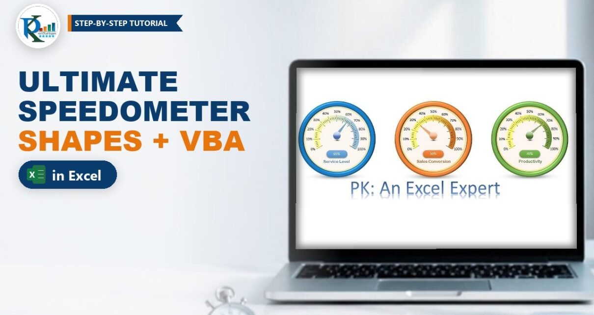
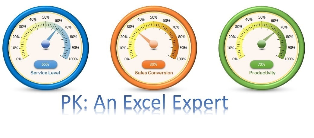
This speedometer in Excel is one of PK’s favourite visuals, and it is not a chart at all. The dial, the coloured arc, the glossy ball and the needle are all ordinary shapes, and a three-line VBA macro turns the needle whenever the value in the cell changes. In this tutorial you will see how each layer is drawn, the simple trick that makes a triangle spin around the centre of the dial, and the Worksheet_Change code that links the needle to your KPI. The finished workbook shows Service Level, Sales Conversion and Productivity side by side.
Watch the Video Tutorial
The build is split into two videos. Part 1 draws the dial, arc, ball, shadow and needle:
Part 2 writes the macro that rotates the needle and adds the scale lines, percentage labels and the value badge:
What You Will Build
- A 3D-looking dial made from an oval with a thick outline and a circle bevel.
- A gradient arc from a Block Arc shape that fades from yellow to the theme colour.
- A needle that pivots on the centre, using a grouped pair of triangles.
- A Worksheet_Change macro that rotates the needle from 0 to 248 degrees as the value goes from 0% to 100%.
- Scale lines, 0% to 100% labels and a linked value badge, so the gauge reads like a real meter.
The Data
The gauges read three percentages in B2:C4:
- B2 Service Level, C2 65%
- B3 Sales Conversion, C3 30%
- B4 Productivity, C4 70%
The video builds the blue Service Level gauge on a new sheet, linked to C2. The other two are made the same way with different colours.
Part 1 – Draw the Speedometer in Excel with Shapes
Step 1: The outer dial
Go to Insert > Shapes > Oval and hold Shift while you drag, so you get a perfect circle. Set Shape Fill to No Fill and pick a blue outline. Right-click > Format Shape and set the line Width to 15 pt. Then open Effects > 3-D Format and choose Circle as the Top bevel. The thick ring now looks like a raised metal rim.
Step 2: The inner face
Insert a second, smaller circle inside the dial. Give it a light fill with about 40-50% transparency, an orange outline and a line width of 2 pt.
Step 3: The coloured arc
Insert a Block Arc (Basic Shapes). Drag its yellow handle to set the band thickness and resize it to sit inside the face. Remove the outline, then in Format Shape choose Gradient fill:
- Delete the extra stops so you have two: one blue (the theme colour) and one yellow.
- Change Type from Radial to Linear and pick the linear left direction.
- Set both stops to 50% transparency so the arc looks soft.
Step 4: The glossy ball and its shadow
Insert a small oval, about 0.5″ x 0.5″, with no outline and a white-to-blue gradient. Add a smaller oval on top with a white-to-white gradient, one stop at 100% transparency and the other at 20-30%, to give the ball a highlight. For the shadow under the ball, add a flat oval with a black-to-white gradient and Type set to Path.
Step 5: The needle
Insert an Isosceles Triangle, make it long and thin, remove the outline and colour it to match the theme.
Part 2 – Make the Needle Rotate Around the Centre
Step 6: The two-triangle pivot trick
If you rotate a single triangle in Format Shape > Size > Rotation, Excel spins it around its own middle, so the needle drifts away from the centre of the dial. PK’s fix:
- Copy the needle and rotate the copy by 180 degrees (Rotate Right 90 degrees, twice).
- Place the copy so the two triangles meet tip to tip, with the meeting point exactly on the centre of the ball.
- Set the copy to No Fill. It is invisible, but it still counts towards the shape’s size.
- Select both triangles and Group them. In the video the group is named
Group 10(you can see the name in the Name Box).
A group rotates around its own centre, which is now the meeting point, so the visible needle swings around the middle of the dial like a real pointer.
Step 7: Find the full-scale angle
Rotate the group so the needle points at 0% and treat that as rotation 0. Then type angles in Format Shape > Size > Rotation until the needle reaches the 100% end of the arc. For this dial that is about 248 degrees, so the needle moves from 0 to 248 degrees as the value goes from 0% to 100%. Your own angle depends on how far your arc wraps, so check it the same way.
Part 3 – The VBA Code That Moves the Needle
Step 8: Add the Worksheet_Change macro
Press Alt+F11, double-click the sheet that holds the gauge, choose Worksheet in the left drop-down and Change in the right one. This is the code from the video:
Private Sub Worksheet_Change(ByVal Target As Range)

ActiveSheet.Shapes.Range(Array("Group 10")).Select
Selection.ShapeRange.Rotation = Range("C2").Value * 248
ActiveCell.Select

End Sub
How the code works
Worksheet_Changeruns automatically every time a cell on this sheet is edited.Shapes.Range(Array("Group 10")).Selectselects the needle group by name.Range("C2").Value * 248turns the percentage into an angle. 65% is stored as 0.65, so the needle turns 0.65 x 248 = about 161 degrees. 0% gives 0 degrees and 100% gives the full 248.ActiveCell.Selectputs the selection back on the cell, otherwise the needle group stays selected after every edit.
Go back to Excel, make sure Design Mode on the Developer tab is switched off, and type 30%, 40% or 100% in C2. The needle jumps to the new value. Right-click the needle group and choose Send to Back so the ball sits on top of it.
Part 4 – Scale Lines, Labels and the Value Badge
Step 9: Scale lines
Here the macro doubles as a ruler. Draw a short black line for the 0% mark. Type 10% in C2 so the needle points to the 10% position, copy the line and rotate it in Format Shape so it lines up with the needle. Repeat for 20%, 30% and so on up to 100%. Then add four thinner lines (width 1 pt) between each pair of big lines.
Step 10: Percentage labels
Insert a text box, type 0%, set it to No Fill and No Line, and place it beside the first big line. Copy it for 10% to 100%.
Step 11: The value badge and caption
Insert a Rounded Rectangle under the ball. With it selected, click in the formula bar, type =$C$2 and press Enter. The badge now shows the live value. Centre the text and make the font white. Add a text box linked to the label cell (Service Level) in the same way, with no fill and no outline.
Step 12: Finishing touches
Turn off gridlines on the View tab. For a standing-on-the-desk look, add a wide flat oval under the dial with a black-to-white Path gradient and high transparency. Build the orange and green gauges the same way, changing only the colours and the linked cell.
Driving All Three Gauges
The video shows the code for the first gauge. For the others you need one more pair of lines per needle, each pointing at its own group and cell. Check each group’s name in the Name Box or the Selection Pane; the names below are only examples. This is an extension of the video’s code, not something shown in it:
Private Sub Worksheet_Change(ByVal Target As Range)
    ' Example group names: replace them with the names in your Name Box
    Me.Shapes("Group 10").Rotation = Range("C2").Value * 248
    Me.Shapes("Group 20").Rotation = Range("C3").Value * 248
    Me.Shapes("Group 30").Rotation = Range("C4").Value * 248
End Sub
Setting Rotation on the shape directly does the same job as selecting it first, so you no longer need ActiveCell.Select.
Common Errors and Fixes
Run-time error 438
The video hits this too: a property name was mistyped (rotaion). Check the spelling of Rotation and ShapeRange.
The needle does not move
Make sure the code is in the sheet’s own module (not a standard module), macros are enabled, Design Mode is off, and the workbook is saved as .xlsm or .xlsb.
Error: the item with the specified name was not found
The name in Array("Group 10") does not match your group. Select the group and read its real name in the Name Box.
The needle wobbles off-centre
The invisible twin triangle is missing or not the same size. Copy the visible needle again so both halves match exactly, then regroup.
Tips
- Rename each group in the Selection Pane (for example NeedleService) so the code is easier to read.
- Values above 100% would push the needle past the arc. Wrap the value with
Application.Min(Range("C2").Value, 1)to cap it (an addition to the original code). - If C2 is a formula, the Change event does not fire when its inputs change elsewhere. Use the
Worksheet_Calculateevent instead. - Microsoft documents the Worksheet.Change event and the Shape.Rotation property used here.
Want It Ready-Made?
The finished workbook with all three gauges, the formatted dials and the working macro is available as the Ultimate Speedometer in Excel on NextGenTemplates.com. For more KPI visuals, browse the Excel charts collection. To learn charts, infographics and full dashboards step by step, see the video course Excel Pivot Tables & Dashboards: Basic to Advanced.
Related Tutorials
- Speedometer Chart in Excel: Build a Gauge Chart Step by Step
- Animated Speedometer Chart in Excel
- 3D Gauge Chart in Excel
- RYG Dial Gauge Meter in Excel
- Advanced Excel Charts and Infographics
Frequently Asked Questions
Can I make a speedometer in Excel without a chart?
Yes. This speedometer uses only shapes: an oval dial, a Block Arc, ovals for the ball and shadow, and a triangle needle. A short VBA macro rotates the needle based on the cell value.
Why does the needle need two triangles?
A shape rotates around its own centre. Grouping the visible needle with an invisible copy turned 180 degrees moves the centre of the group to the tip, so the needle pivots on the middle of the dial.
Where does the number 248 come from?
It is the rotation angle at which the needle points to 100% on this dial. Multiplying the percentage by 248 gives the angle for any value between 0% and 100%. Measure your own dial the same way if your arc is shaped differently.
Does the speedometer update automatically?
Yes, when you type a new value. The Worksheet_Change event runs the code each time a cell on the sheet is edited. If the value comes from a formula, use the Worksheet_Calculate event instead.
Does it work in Excel 365?
Yes. Shapes, gradient fills, 3-D bevels and the Worksheet_Change event all work in current versions of Excel for Windows. Save the file as a macro-enabled workbook and enable macros when you open it.
About the Author
PK is a Microsoft Excel expert and trainer and the founder of PK: An Excel Expert and NextGenTemplates.com. He has been teaching Excel, VBA, Power Query and Power BI since 2016 on his YouTube channel.
Conclusion
A shape-based speedometer in Excel looks far more polished than a standard doughnut gauge, and it needs only a few layers and three lines of VBA. Draw the dial and arc, use the two-triangle trick so the needle pivots on the centre, and multiply the cell value by the full-scale angle. Once the first gauge works, copy it, recolour it and point it at your next KPI.