Excel FIND Function: Syntax, Examples and Tips

Part of the free Module 5: Excel Formulas and Functions · Function 31 of 105 · Full Excel course

The Excel FIND function returns the position of one text string inside another, counting from the first character of the text being searched. The search is case-sensitive and does not accept wildcards. If the text is not found, FIND returns #VALUE!. It is mainly used with LEFT, RIGHT and MID to split text at a known character.

Table of Contents

Syntax

=FIND(find_text, within_text, [start_num])

Arguments

Argument	Required / Optional	Meaning
find_text	Required	The text to look for. An empty string returns the value of start_num (1 by default).
within_text	Required	The text or cell in which to search.
start_num	Optional	The character position at which to begin the search. Default is 1. The returned position is still counted from the start of within_text.

Step-by-step example

The screenshot below shows FIND applied to a list of text values. Follow the same steps in your own workbook.

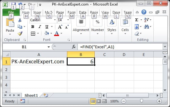
Type a text value such as PK-AnExcelExpert in A2.
In B2 enter =FIND("-",A2). Excel returns 3 because the hyphen is the third character.
In C2 enter =FIND("e",A2). The result is 8, the first lower-case e; the upper-case E in “Excel” is skipped because FIND is case-sensitive.
In D2 enter =FIND("e",A2,9). The search starts at character 9 and returns 11, the next lower-case e.
Fill the formulas down for the remaining rows.

Practical use cases

1. Extract the text before a separator

=LEFT(A2,FIND("@",A2)-1)

Returns the user name from an email address. Subtracting 1 removes the @ itself.

2. Extract the text after a separator

=MID(A2,FIND("@",A2)+1,LEN(A2))

Returns the domain. Using LEN as the length argument avoids calculating the exact remaining count.

3. Pull the second word from a sentence

=MID(A2,FIND(" ",A2)+1,FIND(" ",A2,FIND(" ",A2)+1)-FIND(" ",A2)-1)

The inner FIND locates the first space; the outer FIND starts after it to locate the second space.

4. Test whether text contains a value (case-sensitive)

=ISNUMBER(FIND("USD",A2))

Returns TRUE or FALSE without showing an error when the value is missing.

Common mistakes and tips

#VALUE! error: the text was not found, start_num is 0 or negative, or start_num is larger than the length of within_text. Wrap the formula in IFERROR to return a friendly result.
Case matters: FIND(“a”,”Apple”) returns #VALUE!. Use SEARCH for a case-insensitive match.
No wildcards: the characters * and ? are treated literally. SEARCH supports wildcards; FIND does not.
Position is absolute: even with start_num set to 5, the result counts from character 1 of the string.
Numbers: both arguments are converted to text, so FIND(5,12345) returns 5.

FIND with IFERROR, SEARCH and SUBSTITUTE

Because FIND returns #VALUE! when the text is missing, production formulas normally wrap it. =IFERROR(LEFT(A2,FIND("-",A2)-1),A2) returns the text before the hyphen, or the whole text when there is no hyphen, so the column never shows errors. When case does not matter, swap FIND for SEARCH with the same three arguments; the two functions are otherwise interchangeable. To count how many times a character occurs, use =LEN(A2)-LEN(SUBSTITUTE(A2,"-","")), which avoids FIND altogether. To locate the last occurrence of a character, a task FIND cannot do directly, replace that occurrence with a unique marker first: =FIND("#",SUBSTITUTE(A2,"/","#",LEN(A2)-LEN(SUBSTITUTE(A2,"/","")))) returns the position of the final slash in a file path.

Related functions

SEARCH: the case-insensitive version that also accepts wildcards.
MID: extracts text from a position that FIND supplies.
LEFT: returns the characters before the found position.
LEN: gives the string length used in extraction formulas.
See all lessons in the Excel Formulas course.

Frequently asked questions

What is the difference between FIND and SEARCH in Excel?

FIND is case-sensitive and does not support wildcards. SEARCH ignores case and accepts the wildcards * and ?. Both return the position of the first match.