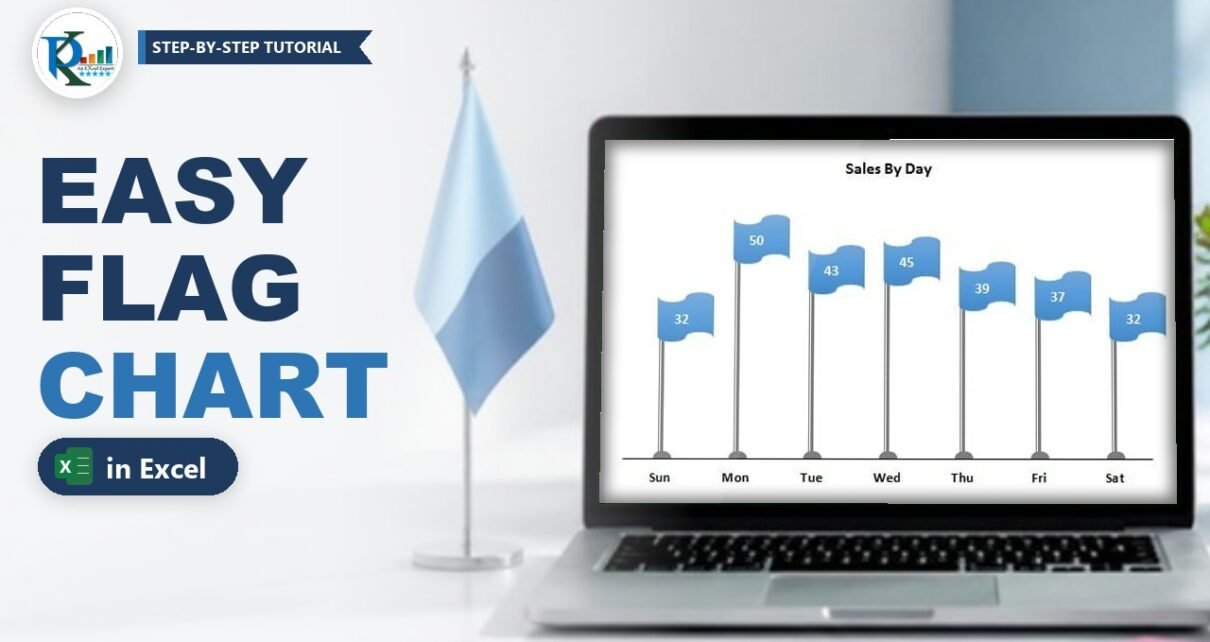
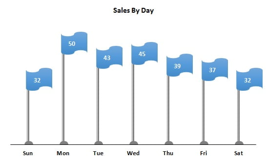
A flag chart in Excel turns a plain column chart into an eye-catching infographic: every value becomes a flag on a pole, and the pole height shows the number. It works best with a small data set, such as sales by day of the week. In this tutorial you build it from scratch with three ordinary Excel tools: a 2-D clustered column chart, error bars that draw the poles, and an auto shape that becomes the flag. You also learn a small REPT trick that centres each value on its flag.
Watch the Video Tutorial
In the video PK starts from the day-wise sales table, turns the columns into poles with error bars, pastes a Punched Tape shape onto a line series to create the flags and finishes with centred data labels.
What You Will Build
- Grey poles drawn by minus error bars at 100%, with a round foot made by the oval arrow end.
- Invisible columns that only exist to carry the error bars.
- Blue flags made from the Flowchart: Punched Tape shape, pasted as the markers of a line series.
- Centred value labels on every flag, using a helper column with the REPT function.
- A clean look with no gridlines, no vertical axis and only the day names at the bottom.
The Data Set
The example uses one week of sales. Day names are in A2:A8 and the sales values in B2:B8, with the headers Day and Sales in row 1:
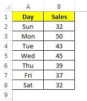
Seven values is the sweet spot. With many more categories the flags get crowded, and a normal column chart is easier to read.
Part 1 – Build the Flag Chart Poles
Step 1: Remove the gridlines and insert a column chart
First switch off the sheet gridlines (View → Gridlines) so the finished chart sits on a clean background. Then select A1:B8 and go to Insert → Charts → Column → 2-D Clustered Column.
Step 2: Add minus error bars at 100%
Click any column, then the Chart Elements button (the plus icon), point to Error Bars, click the arrow and choose More Options. In the Format Error Bars pane set:
- Direction: Minus
- End Style: No Cap
- Error Amount: Percentage, 100%
A minus error bar of 100% starts at the top of each column and runs all the way down to zero. In other words, it is exactly as tall as the value, which is what a flag pole needs.
Step 3: Style the error bars as poles
Still in the error bar pane, open Fill & Line and choose:
- Line: Solid line, colour dark grey
- Width: 4.5 pt
- Compound type: Thick Thin (the double line gives the pole a metallic edge)
- End arrow type: Oval – this draws the round foot at the bottom of every pole
Step 4: Hide the columns, the axis and the gridlines
Click the columns and on the Format tab set Shape Fill → No Fill. Only the poles stay visible. Then click the vertical axis and press Delete, and do the same for the chart gridlines.
Part 2 – Turn a Line Series into Flags
Step 5: Add the same data as a second series
You need a second series with the same values to carry the flags. You can right-click the chart, choose Select Data → Add and pick the Sales range again, but the quicker way PK shows is: select A1:B8, press Ctrl + C, click the chart and press Ctrl + V. A second (orange) series appears.
Step 6: Change the new series to a line with markers
Right-click the new series, choose Change Series Chart Type and set it to Line with Markers. Its points now sit exactly at the top of each pole.
Step 7: Draw the flag shape
Go to Insert → Shapes and, under Flowchart, pick Punched Tape. Its wavy top and bottom edges look like a flag in the wind. Click on the sheet to draw it, apply a blue shape style from the Format tab and resize it so it is small enough for the chart.
Step 8: Add an invisible partner so the flag sits beside the pole
Copy and paste the flag to get a second copy. Set the copy to Shape Fill → No Fill and Shape Outline → No Outline, select both shapes, right-click and choose Group.
Why the invisible copy? Excel always centres a picture marker on the data point. When the group contains the blue flag plus an invisible shape, the centre of the group can sit on the pole while the visible flag hangs to one side of it.
Step 9: Paste the group onto the line series
Copy the group, click the line series once (so all its points are selected) and press Ctrl + V. Every marker becomes a flag. If a flag still covers its pole, select the blue flag inside your original group, nudge it to the left three or four times with the arrow key, then copy the group and paste it onto the series again until the flags fly from the top of the poles.
Step 10: Hide the connecting line
Right-click the line series, choose Format Data Series → Fill & Line → Line → No line. The orange line between the flags disappears and only the flags remain.
Part 3 – Centre the Values on the Flags
Step 11: Add data labels
Right-click the flags, choose Add Data Labels, then Format Data Labels and set Label Position to Center. The numbers appear, but because the flag hangs to the side of the data point, they sit on the pole instead of in the middle of the flag.
Step 12: Build a padded label column with REPT
The fix is to push the text to the right with leading spaces. Type the number of spaces you want in C1, then enter this in C2 and fill it down to C8:
C2 =REPT(" ",$C$1)&B2How the formula works
REPT(" ",$C$1)repeats a single space as many times as the number in C1.&B2joins the sales value after those spaces, so C2 shows the number shifted to the right.$C$1is locked with F4, so every row uses the same number of spaces when you fill the formula down.
Step 13: Use the helper column as the label source
In Format Data Labels → Label Options tick Value From Cells, select C2:C8 and click OK. Untick Value and Show Leader Lines. Make the labels bold, black and a little bigger.
Now tune C1. With 5 the numbers were still slightly to the left; in the video PK settles on 12, which puts every value neatly in the middle of its flag. Because the labels read from cells, changing C1 moves all of them at once.
Value From Cells exists in Excel 2013 and later. In Excel 2010 and older you would have to click each label and link it to its cell one by one.
Add a chart title such as Sales By Day and your flag chart is ready.
Common Errors and Fixes
These fixes are general Excel guidance added to this refresh.
The poles do not reach the axis
The error amount is not 100% or the direction is Both or Plus. Set Direction to Minus and Percentage to 100.
The flags appear on only one point
You clicked a point twice, which selects a single point. Click the line series once so all points are selected, then paste.
The labels change when you edit the sales values
That is expected: the REPT column reads from B2:B8, so the labels follow your data. If they show the old value, check that C2:C8 is still the Value From Cells range.
The flags look stretched or too large
Resize the original shapes, regroup them and paste the group onto the series again. Excel uses the pasted picture at its current size.
Tips
These tips are extras added to this refresh; they are not shown in the video.
- Keep the flags one colour for a clean look, or paste a differently coloured flag onto a single point (click the series, then click one point) to highlight the best day.
- Try other flag-like shapes, such as a wave or a pennant drawn with a triangle, using the same grouping trick.
- Save the finished chart as a chart template (right-click the chart, Save as Template) to reuse the poles and styling.
- Use the flag chart for 5 to 10 categories; beyond that the flags overlap.
- Microsoft's guide to adding error bars in a chart explains every error bar option used here.
Want It Ready-Made?
If you would rather use a finished, editable version, the Flag Chart in Excel template is available on NextGenTemplates.com, together with many more Excel charts and visualizations. To learn charts, infographics and dashboards step by step, join the course Excel Pivot Tables & Dashboards: Basic to Advanced on NextGenTemplates Academy.
Related Tutorials
- Conditional Formatting in a Lollipop Chart in Excel
- Balloon Chart in MS Excel
- Info-graphics with Column Chart (Part 1)
- How to Use the Picture Effect in Your Chart
- Column Chart in Excel
Frequently Asked Questions
What is a flag chart in Excel?
It is an infographic version of a column chart. Each category gets a pole whose height equals its value and a flag at the top that shows the number. It is built from a clustered column chart, error bars and a shape.
Which chart type do I start with?
Start with a 2-D clustered column chart. The columns are later made invisible and only carry the error bars that draw the poles, while a second series changed to a line with markers carries the flags.
How do the error bars become flag poles?
Set the error bars to Minus, No Cap and a 100 percent error amount. They then run from the top of each column down to zero, which is exactly the pole height. A solid grey line, Thick Thin compound type and an oval end arrow finish the look.
Why do I group the flag with an invisible shape?
Excel centres a picture marker on the data point. Grouping the visible flag with a transparent copy moves the visible part to one side, so the flag hangs from the pole instead of covering it.
How do I put the numbers in the middle of the flags?
Create a helper column that adds leading spaces in front of each value with the REPT function, as shown in Step 12, and use it as the label source with Value From Cells. Change the number of spaces until the labels sit in the centre.
Can I download the flag chart template?
A ready-made, editable Flag Chart in Excel template is available on NextGenTemplates.com. You can also build it yourself in a few minutes with the steps above.
About the Author
PK is a Microsoft Excel expert and trainer and the founder of PK: An Excel Expert and NextGenTemplates.com. He has been teaching Excel, Power Query and Power BI since 2016 on his YouTube channel.
Conclusion
A flag chart in Excel is a simple column chart in disguise: minus error bars at 100% draw the poles, a line series wearing a Punched Tape shape carries the flags, and a REPT helper column centres the values. Build it once with the week's sales, save it as a template, and you have an eye-catching chart ready for your next presentation or dashboard.