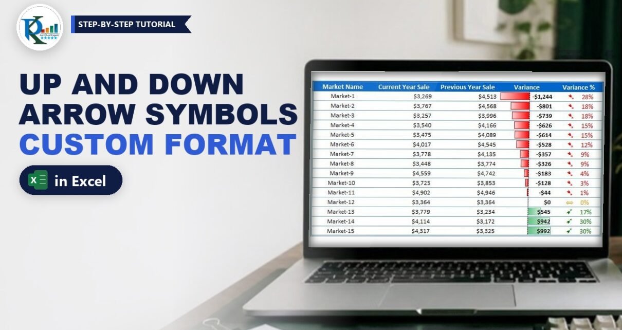
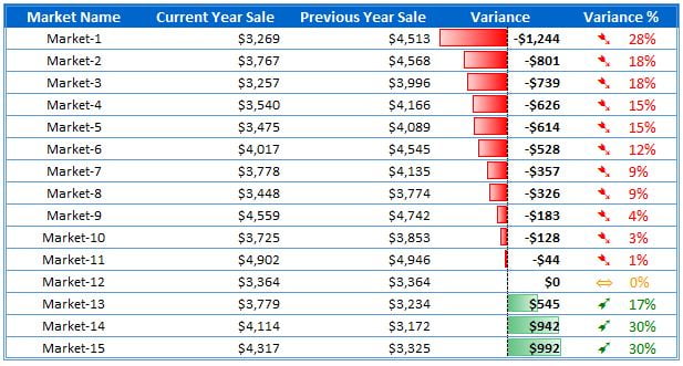
Arrow symbols in Excel with custom formatting let you show a coloured up or down arrow right next to a percentage, without a single extra formula or helper column. In this tutorial you take a market-wise sales table for the current and previous year, calculate the variance and the variance %, add red and green data bars to the variance, and then use one custom number format that shows a green up arrow for growth, a red down arrow for decline and an orange two-way arrow for no change.
⬇️ Download the Practice File
.xlsx workbook (21 KB) · Excel 2013 and later for Windows · no macros
Watch the Video Tutorial
In the video, PK rebuilds the table on a new sheet, adds red and green data bars, picks arrows from a UNICHAR code list and fine-tunes the custom format with spacing, indent and colour index numbers.
What You Will Build
- A sales comparison table with Market Name, Current Year Sale, Previous Year Sale, Variance and Variance %.
- Red and green data bars that show negative and positive variance at a glance.
- A green up arrow for markets that grew, a red down arrow for markets that dropped and an orange two-way arrow for no change.
- One custom number format that does all of this, so the cell still holds a real number you can sort, filter and use in formulas.
- A reusable list of arrow characters built with the UNICHAR function.
How the Practice File Is Laid Out
The download has three sheets:
- Custom Formatting: the finished table in C5:G20, with Market-1 to Market-15.
- Sheet4: the same table that PK builds step by step in the video (D4:H19).
- Unichar: two lists of Unicode codes with the character each one returns, so you can pick the arrow you like.
The steps below use the cell references of the Custom Formatting sheet: headers in row 5 and data in rows 6 to 20.
Part 1: Calculate the Variance and Variance %
Step 1: Set up the table
Type the five headers in C5:G5 and enter the market names and the two sales columns below them. Turn off gridlines with View > Gridlines and add a border with Format Cells (PK uses the shortcut Alt, O, E, then the Border tab).
Step 2: Calculate the variance
The variance is the current year sale minus the previous year sale. In F6 enter:
=D6-E6Fill it down to F20 and give it a currency format such as "$"#,##0. Market-1 sold $3,269 this year against $4,513 last year, so its variance is -$1,244.
Step 3: Calculate the variance %
The variance % compares the change with the previous year. In G6 enter:
=(D6-E6)/E6Fill it down and format it as a percentage. In the video PK writes it as =G5/F5 on Sheet4, which is the same thing: the variance divided by the previous year sale. Market-1 gives -28%, Market-12 gives 0% and Market-15 gives 30%.
Part 2: Add Red and Green Data Bars
Step 4: Apply a gradient data bar
Select the variance values F6:F20 and go to Home > Conditional Formatting > Data Bars > Gradient Fill and pick the green bar (the second option). Excel draws positive values as green bars to the right of an axis and negative values as red bars to the left, so you get the red and green look without any extra rule.
The longest red bar marks the biggest drop (Market-1) and the longest green bar the biggest gain. If you sort the table by Variance, the bars line up from the biggest loss to the biggest gain, which reads very well in a report.
Part 3: Arrow Symbols in Excel with Custom Formatting
Step 5: Pick your arrows with UNICHAR
Excel can return any Unicode character from its code with the UNICHAR function. On the Unichar sheet, A1 holds 8592 and each cell below adds 1, while column B shows the character:
=UNICHAR(A1)Column F does the same from 10136 to 10174, which is a block of designer arrows. The three arrows used in the final table are:
- ➹ (code 10169) for an increase
- ➷ (code 10167) for a decrease
- ⇔ (code 8660) for no change
To use one, copy the cell, paste it as a value (so it becomes the plain character, not a formula), then copy that character so you can paste it into the format code.
Step 6: Understand the four sections of a custom format
Select G6:G20 and open Format Cells > Number > Custom. A custom number format can have up to four sections separated by semicolons, always in this order:
positive ; negative ; zero ; textExcel uses the first section for positive numbers, the second for negative numbers and the third for zero. You don’t need the text section here, so you can leave it out.
Step 7: Write the arrow format
In each section you put a colour in square brackets, the arrow inside double quotes, and then the number format. With named colours, the format looks like this (in the video PK starts this way, then swaps in better arrows):
[Green]"➹"0%;[Red]"➷"0%;[Yellow]"⇔"0%It works, but the green is very light and the yellow is hard to read on white. The final format in the practice file is:
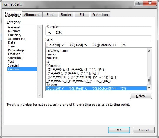
[Color10]"➹ "0%;[Red]"➷ "0%;[Color45]"⇔ "0%How the format works
- [Color10]”➹ “0%: positive numbers turn dark green and get the up arrow, five spaces and the percentage.
- [Red]”➷ “0%: negative numbers turn red with the down arrow. There is no minus sign in this section, so -28% shows as 28%. The red colour and the down arrow already tell you it is a decline.
- [Color45]”⇔ “0%: zero shows in orange with the two-way arrow.
- 0% shows whole percentages. Use
0.0%if you want one decimal place. - The cell value does not change. G6 still holds -0.2756, so sorting, filtering and formulas keep working.
Step 8: Choose readable colours with colour index numbers
Besides the eight named colours (such as Red, Green and Yellow), a custom format accepts [ColorN], where N is a number from 1 to 56 from Excel’s colour index palette. In the video PK checks the 56 colour index list and picks:
- Color10: a dark green that is easy to read (43 and 51 are other options).
- Color45: an orange or amber for zero (44 also works).
- Red stays as it is, because it is already clear (Color3 gives the same red).
Step 9: Space and align the arrows
Two finishing touches make the column look neat:
- Type five spaces after each arrow, inside the quotes, so there is a gap between the arrow and the number.
- Left-align G6:G20 and click Home > Increase Indent a couple of times. All arrows now start at the same position and the percentages line up beneath each other.
Make the column bold if you like, and the table is ready to drop into a dashboard.
Alternative: Conditional Formatting Icon Sets
This section is an addition and is not in the original file or video. Excel also has built-in arrows under Home > Conditional Formatting > Icon Sets. Pick the 3 Arrows set, then use Manage Rules > Edit Rule and switch the type to Number so the green arrow shows for values above 0 and the red arrow for values below 0. Icon sets are quick, but you can’t change their colours or style, and they ignore the number format. The custom format method gives you any arrow and any colour, and the arrows travel with the cell when you copy the format with Format Painter.
Common Errors and Fixes
The arrows show as empty boxes
The font in the cell doesn’t include that character. Calibri, Arial and Segoe UI Symbol show these arrows on Windows. Change the font of the column or choose a different arrow code from the Unichar list.
Excel says the number format is not valid
Check that each arrow is inside straight double quotes, that each colour is in square brackets, and that the sections are separated by semicolons, not commas.
The arrow appears but the colour is wrong
The sections are in the wrong order. Excel always reads positive first, then negative, then zero.
Nothing changes in some cells
Those cells hold text, not numbers (for example a percentage typed with an apostrophe). Number formats only affect numbers, so convert the values back to numbers.
Tips
- Keep the Unichar sheet in your personal toolkit so you can pick symbols for any future report.
- If you only want the arrow and no number, leave out the number code in each section, as PK mentions in the video.
- Combine the arrows with the data bars: the bars show size, the arrows show direction.
- Microsoft lists every code you can use in its guidelines for customizing a number format, and explains the UNICHAR function.
Want It Ready-Made?
If you want variance arrows in a chart instead of a table, the Dynamic Variance Arrows Chart with Slicers is ready to use, and you can browse more Excel chart templates on NextGenTemplates.com. To learn conditional formatting, charts and dashboard design step by step, take a look at the Excel Pivot Tables and Dashboards course.
Related Tutorials
- Transform Excel Data with Arrows and Color Coding with Custom Formatting
- Highlight Sales Figures with Custom Number Formatting in Excel
- Dynamic Number Format for Millions and Thousands
- Multi-color Data Bar with the REPT Function
- Symbols and Emojis in Excel Drop-down Lists and Charts
Frequently Asked Questions
How do I add up and down arrows to percentages in Excel?
Select the cells, open Format Cells, choose Custom and enter a format with three sections: a colour, the up arrow and 0% for positive values, then a colour, the down arrow and 0% for negative values, then a colour, a neutral arrow and 0% for zero. Step 7 shows the exact code.
Does custom formatting change the value in the cell?
No. A custom number format only changes how the value looks. The cell still holds the original number, so you can sort, filter and calculate with it.
Why does a negative percentage show without a minus sign?
The negative section of the format has no minus sign, so Excel shows the value without it. The red colour and the down arrow show the decline instead. Add a minus sign before 0% in the second section if you want it.
What do Color10 and Color45 mean in a number format?
They are colour index numbers from the 56 colour palette of Excel. Color10 is a dark green and Color45 is an orange. You can use any number from 1 to 56 in square brackets.
How do I find the code of an arrow symbol?
Use the UNICHAR function with a list of numbers, as on the Unichar sheet of the practice file. Codes 8592 to 8703 and 10136 to 10174 contain many arrow styles.
About the Author
PK is a Microsoft Excel expert and trainer and the founder of PK: An Excel Expert and NextGenTemplates.com. He has been teaching Excel, VBA, Power Query and Power BI since 2016 on his YouTube channel.
Conclusion
Arrow symbols in Excel with custom formatting are one of the easiest ways to make a variance report speak for itself. Calculate the variance and the variance %, add gradient data bars for the size of the change, and use one custom format with a colour, an arrow and 0% for each section. Choose readable colours with Color10 and Color45, add a little spacing and indent, and your table is ready for any dashboard. Download the practice file and try it with your own numbers.