Slicers in Pivot Table: Insert, Connect, Columns

Part of the free Module 10: Pivot Tables · Lesson 10 of 20 · Full Excel course

Updated on 5 September 2026 · Works in Excel 365, 2021, 2019 and 2016 unless noted.

A slicer in a pivot table is a floating panel of filter buttons that shows at a glance which items are selected. You insert one from PivotTable Analyze > Insert Slicer, click a button to filter, and use Report Connections to make the same slicer drive several pivot tables and pivot charts at once. Slicers exist in Excel 2010 and every later version, including Excel for the web.

Slicer, report filter and timeline compared

All three tools filter the same pivot table, but they suit different jobs. Choose by how visible the selection has to be and by whether more than one report must react.

Feature	Slicer	Report Filter	Timeline
Selection visible without clicking	Yes, every item is a button	No, hidden in a drop-down	Yes, a highlighted date band
Field types accepted	Text, number and date fields	Any field	Real date fields only
Controls several pivot tables	Yes, through Report Connections	No	Yes, through Report Connections
Works on an Excel Table	Yes, from Excel 2013	No	No
Screen space used	Large, but resizable and stylable	One row above the report	One horizontal bar
Best for	Dashboards and shared workbooks	Compact printed reports	Filtering by month, quarter or year

Report filters are covered in the lesson on pivot table filters, and the date-only twin of the slicer is explained in the timeline lesson.

How to insert a slicer in a pivot table

Click anywhere inside the pivot table so the PivotTable tools appear on the ribbon.
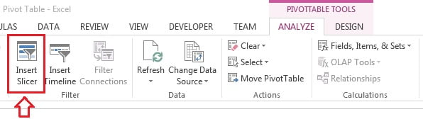
On the PivotTable Analyze tab click Insert Slicer in the Filter group. The command also sits on the Insert tab under Filters > Slicer. In Excel 2010 and 2013 the tab is called Options under PivotTable Tools.

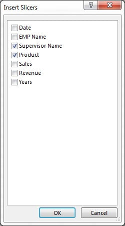
Insert Slicer button in the Filter group of the PivotTable Analyze tab used to add slicers in a pivot table — Insert Slicer on the PivotTable Analyze tab

In the Insert Slicers dialog tick each field you want buttons for, for example Supervisor Name and Product, then click OK. Excel creates one slicer per ticked field, so tick only the two or three fields people will actually use.

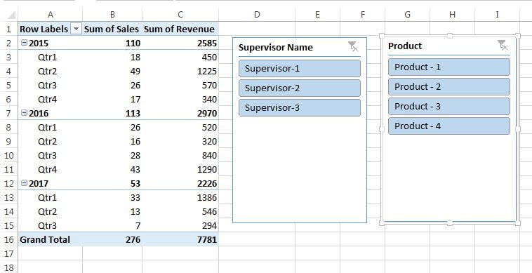
Insert Slicers dialog listing every pivot table field with a check box beside it — Insert Slicers dialog

The slicers land stacked on the worksheet. Drag each one by its header to position it and use the corner handles to resize it.

Supervisor and Product slicers placed beside a pivot table in the worksheet — Slicers inserted next to the pivot table

Select single and multiple items, and clear the filter

One click on a button filters the report to that item. Items that return no rows under the current selection are greyed out and pushed to the bottom of the list, which is a fast way to spot combinations that have no data.

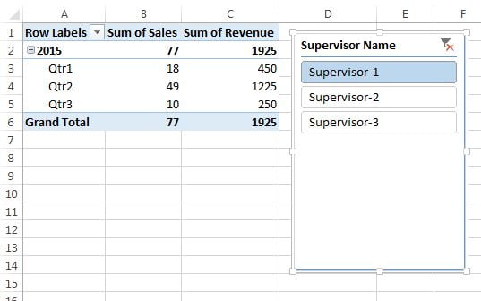
Click Supervisor-1 to keep only that supervisor.
Hold Ctrl and click more buttons to add them to the selection. Ctrl-clicking a selected item removes it again.
In Excel 2016 and later click the Multi-Select icon in the slicer header, or press Alt + S while the slicer is selected, so that every plain click toggles an item without holding Ctrl. This is the setting to use on touch screens.
Click the Clear Filter icon in the top right of the slicer, or press Alt + C, to show all items again.
Drag across adjacent buttons, or click the first and Shift-click the last, to select a block of items in one movement.

Pivot table filtered to Supervisor-1 by clicking that item in the slicer — Pivot table filtered by Supervisor-1 through the slicer

Connect one slicer to several pivot tables

This is the step that turns two separate reports into a dashboard. A slicer can control every pivot table and pivot chart that shares its pivot cache, which means they were built from the same range or Table in one session, or from the same Data Model.

Name your pivot tables first under PivotTable Analyze > PivotTable Name, using names such as pvtBySupervisor and pvtByProduct, otherwise the dialog only shows PivotTable1, PivotTable2 and so on.
Right-click the slicer and choose Report Connections. The same command sits on the Slicer tab in the Slicer group.

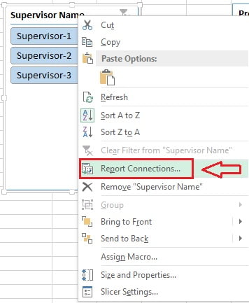
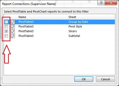
Right-click menu of a slicer showing the Report Connections command — Report Connections in the slicer right-click menu

Tick every pivot table the slicer should drive and click OK. Sheet names are shown beside each pivot table, so a slicer on the dashboard sheet can control reports living on hidden sheets.
Click a button and check that all connected reports and their pivot charts move together.

Report Connections dialog with a check box for each pivot table the slicer can control — Report Connections dialog

Slicer Settings: caption, sorting and empty items

Right-click the slicer and choose Slicer Settings to control how the panel looks and what it lists.

Setting	What it does
Caption	The heading shown on the slicer. Change it to a friendly label such as Sales Region without renaming the source field.
Display header	Untick to hide the caption and the two icons. Do this only after the layout is final, because you also lose the Clear Filter button.
Item sorting	Ascending, descending, or the workbook custom list, which is how month names appear in calendar order instead of April first.
Hide items with no data	Removes greyed-out buttons completely so the panel stays short.
Visually indicate items with no data	Keeps them visible but greyed, which tells the reader that the combination exists but is empty.
Show items deleted from the data source	Untick this to drop items that no longer exist in the source. They survive in the pivot cache and keep appearing until the cache is cleared.

Buttons, columns and locking the slicer in place

A slicer lists items in one column by default. For a field with four or five items a horizontal layout wastes far less space on a dashboard.

Select the slicer and open the Slicer tab, called Slicer Tools > Options before Excel 2019.
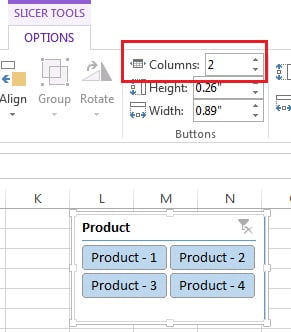
In the Buttons group set Columns to 2. Product-1 and Product-2 now sit on the first row and Product-3 and Product-4 on the second.
Adjust the button Height and Width in the same group, then the slicer Height and Width in the Size group, so no button text is cut off.

Product slicer arranged in two columns using the Columns setting on the Slicer tab — Slicer buttons arranged in two columns

Slicers drift and shrink when rows or columns are hidden or resized. To pin one down, right-click it, choose Size and Properties, expand Properties and select Do not move or size with cells. To stop users dragging it at all, tick Disable resizing and moving in Slicer Settings and then protect the sheet.

Slicers on an Excel Table

From Excel 2013 a slicer can also filter an ordinary Excel Table, no pivot table needed. Click inside the Table, then use Table Design > Insert Slicer or Insert > Filters > Slicer. The buttons drive the Table AutoFilter, so any formula that reads the Table with SUBTOTAL or AGGREGATE updates as you click. A Table slicer cannot be connected to pivot tables, because it filters rows rather than a pivot cache.

Worked example: one Date slicer driving two reports

Use this small extract of the practice data.

Date	Supervisor	Product	Revenue
05-Jan	Supervisor-1	Product-1	4,200
18-Jan	Supervisor-2	Product-3	6,150
03-Feb	Supervisor-1	Product-2	3,800
22-Feb	Supervisor-3	Product-1	5,400

Build the first pivot table with Supervisor in Rows and Sum of Revenue in Values, and name it pvtBySupervisor.
Copy that pivot table to a blank area and swap Supervisor for Product. Copying is what keeps both reports on one pivot cache. Name it pvtByProduct.
Click the first pivot table and insert a Product slicer.
Right-click the slicer, open Report Connections and tick pvtByProduct as well.
Click Product-1. Supervisor-1 shows 4,200 and Supervisor-3 shows 5,400, while the product report reduces to a single row of 9,600. Press Alt + C and both return to the full 19,550.

Errors and how to fix them

Problem	Cause	Fix
The slicer does not appear in Report Connections	The second pivot table was created from scratch, so it has its own pivot cache	Delete it and copy the first pivot table instead, or rebuild both on the same Excel Table, or add both tables to the Data Model
Insert Slicer is greyed out	The cursor is outside the pivot table, the workbook is in Compatibility Mode as an xls file, or the sheet is protected	Click inside the report, save as xlsx and unprotect the sheet
Old items keep showing as greyed buttons	Deleted source items are retained in the pivot cache	Untick Show items deleted from the data source in Slicer Settings, or set Number of items to retain per field to None in PivotTable Options and refresh
The slicer shrinks or moves when columns are hidden	The default object placement is Move and size with cells	Size and Properties > Properties > Do not move or size with cells
Clicking the slicer changes only one report	The other pivot tables were never ticked in Report Connections	Reopen Report Connections and tick every report the slicer should drive
Dates sort as text in the slicer	The date column is stored as text	Convert the column to real dates, refresh, and use a timeline instead

Tips and common mistakes

Copy, do not rebuild. Copying an existing pivot table keeps the shared cache that Report Connections depends on, and it keeps the file smaller.
Name every pivot table. A Report Connections list of PivotTable1 to PivotTable7 is unusable on a real dashboard.
Two or three slicers is the limit. More buttons than data on screen makes a report feel slow and cluttered.
Use a timeline for dates. A slicer on a date field lists every single day, so switch to a timeline for month, quarter or year filtering.
Hide the source sheets, not the slicers. Slicers keep working when the pivot tables they control sit on hidden sheets.
Match the style. Slicer Styles on the Slicer tab align the buttons with your pivot table theme; custom styles are covered in the styles lesson.
Refresh does not break connections. Changing the data source, however, can drop a slicer if the field is renamed, so keep header names stable.

Practice exercise

Open the practice file at Pivot-Table.xlsx and build a supervisor-wise revenue pivot table named pvtBySupervisor.
Copy it, change the row field to Product and name the copy pvtByProduct.
Insert Product and Supervisor Name slicers, then connect both slicers to both pivot tables.
Set the Product slicer to two columns, change its caption to Product Line and sort it descending.
Lock both slicers with Do not move or size with cells, hide the source sheet and confirm the buttons still filter correctly.

Key takeaways

Insert a slicer from PivotTable Analyze > Insert Slicer or Insert > Filters > Slicer.
Ctrl-click or the Multi-Select icon selects several items; Alt + C clears the filter.
Report Connections links one slicer to many pivot tables, but only when they share a pivot cache or the Data Model.
Slicer Settings controls the caption, sorting, empty items and deleted items.
Columns and button size shape the panel; Size and Properties stops it moving with cells.
Excel Tables accept slicers from Excel 2013, and dates are better served by a timeline.

Related lessons

Frequently asked questions

Can one slicer control pivot tables on different sheets?

Yes. Report Connections lists every pivot table in the workbook that shares the slicer pivot cache, whatever sheet it sits on, and it shows the sheet name beside each report. The slicer itself can be cut and pasted onto a dashboard sheet while the pivot tables stay on hidden data sheets.

Why is a pivot table missing from Report Connections?

It was built as a fresh pivot table, so Excel gave it a separate pivot cache and the slicer cannot reach it. Delete it and copy the first pivot table instead, or build every report from the same Excel Table, or load both tables into the Data Model so they share one cache.

How do I select multiple items in a slicer?

Hold Ctrl while clicking each button. In Excel 2016 and later you can instead click the Multi-Select icon in the slicer header, or press Alt + S, so that a plain click toggles an item on or off. Press Alt + C or click the Clear Filter icon to reset the slicer.

What is the difference between a slicer and a report filter?

A report filter is a drop-down above the pivot table, so you must open it to see the selection and it can drive only its own report. A slicer shows every item as a visible button, greys out empty items and can be connected to many pivot tables and pivot charts at once.

Do slicers slow down a workbook?

A few slicers on a normal dataset are fast. Cost rises with the number of items, the number of connected pivot tables and the size of the pivot cache. Hide items with no data, keep slicers to two or three fields, and prefer a timeline over a slicer on a daily date field.

Want the finished version? Ready-made Excel dashboards, trackers and VBA systems are available at NextGenTemplates.com.