Highlight and Count Birthdays from Date of Birth in Excel

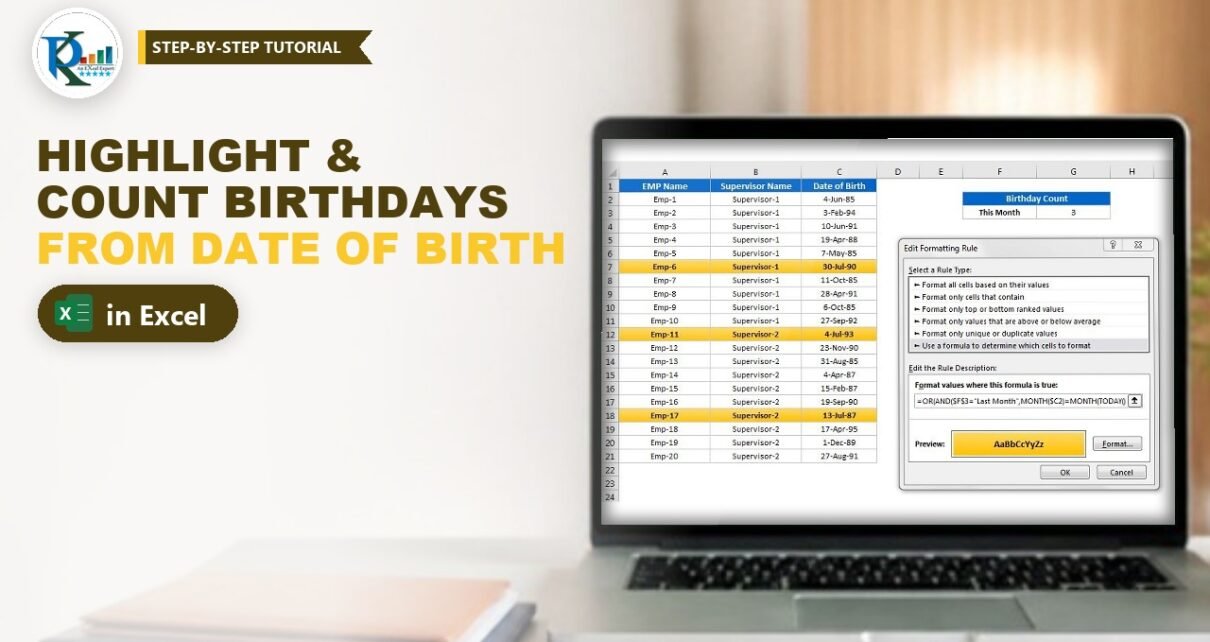
Want to count birthdays from date of birth in Excel and highlight who is celebrating this month? In this tutorial you build a small birthday tracker from a plain employee list. A drop-down lets you pick Last Month, This Month or Next Month, one formula counts the matching birthdays, a second table shows the count for every month, and conditional formatting highlights the matching rows. There is no helper column, no VBA and no user-defined function, only SUM, IF, MONTH, TEXT and TODAY. This tip started as a viewer question: how many people are born in a given month?

⬇️  Download the Birthday Count Practice File
Single-sheet workbook · .xlsx (no macros) · Excel 2007 and later

Watch the Video Tutorial

PK rebuilds the tracker on a new sheet: the month-wise count with SUM, IF and TEXT, the drop-down count with MONTH and TODAY, and the dynamic conditional formatting rule, testing each formula as he goes.

What You Will Build

• A drop-down in F3 with three choices: Last Month, This Month and Next Month.
• A birthday count in G3 that changes with the drop-down and with today’s date.
• A month-wise table (Jan to Dec) that counts birthdays in each month straight from the Date of Birth column.
• Row highlighting for every employee whose birthday falls in the selected month.
• All of it with no helper column: every formula reads the dates directly.

Step 1: Set Up the Employee Data

The practice file has one sheet called Birthday Count with 20 employees:

• A1:A21 – EMP Name (Emp-1 to Emp-20).
• B1:B21 – Supervisor Name (Supervisor-1 and Supervisor-2).
• C1:C21 – Date of Birth, stored as real Excel dates and shown in the d-mmm-yy format, for example 4-Jun-85.

The dates must be real dates, not text. Every formula below pulls the month out of the date, and that only works when Excel sees a number behind the cell.

Step 2: Count Birthdays by Month Name

Build the month list

In F9 type Month and in G9 type Count. Type Jan in F10 and drag the fill handle down to F21. Excel fills the month names through Dec for you.

Enter the counting formula

In G10 enter:

=SUM(IF(TEXT($C$2:$C$21,"MMM")=F10,1,0))

Lock the date range with F4 so it stays fixed when you copy the formula down. In Excel 2019 and earlier, confirm it with Ctrl+Shift+Enter, not just Enter. In the video, plain Enter returns 0, and Ctrl+Shift+Enter adds curly braces around the formula and returns the right count. Then select G10:G21 and press Ctrl+D to fill it down.

How the formula works

• TEXT($C$2:$C$21,"MMM") turns each date into its three-letter month name: 4-Jun-85 becomes Jun, 3-Feb-94 becomes Feb.
• =F10 compares every one of those names with the month in the row, giving 20 TRUE or FALSE results.
• IF(...,1,0) turns each TRUE into 1 and each FALSE into 0.
• SUM adds the ones, which is the number of birthdays in that month.

PK shows a neat trick to see this: click in the formula bar, select the part inside SUM and press F9. For Feb you see an array like {0;1;0;0;…}: the second date (3-Feb-94) gives 1 and the non-February dates give 0. Press Esc afterwards so you do not keep the calculated values.

Step 3: Count Birthdays for Last, This and Next Month

Add the drop-down

Merge F2:G2 and type the heading Birthday Count. Select F3 and open Data → Data Validation (PK uses the shortcut Alt, D, L). Choose List and type the source as:

Last Month,This Month,Next Month

Click OK, and F3 now shows a drop-down arrow. If you are new to this, see the guide on how to create a drop-down list with Data Validation.

Start with this month only

PK builds the formula in two stages. First, a version that only counts this month:

=SUM(IF(MONTH($C$2:$C$21)=MONTH(TODAY()),1,0))

MONTH returns the month number (1 to 12) of each date, and MONTH(TODAY()) returns the current month number. The video was recorded in July, so this returns 3. It does not react to the drop-down yet, because F3 is not in the formula.

Connect the drop-down

Replace MONTH(TODAY()) with a nested IF that picks the target month from F3. The final formula in G3 is:

=SUM(IF(MONTH($C$2:$C$21)=IF(F3="Last Month",MONTH(TODAY())-1,IF(F3="Next Month",MONTH(TODAY())+1,MONTH(TODAY()))),1,0))

Confirm it with Ctrl+Shift+Enter in older Excel versions.

How the formula works

• If F3 is Last Month, the target is the current month number minus 1.
• If F3 is Next Month, the target is the current month number plus 1.
• Otherwise (This Month), the target is the current month number.
• Each birth month is compared with that target, IF turns matches into 1, and SUM counts them.

In the video (July), the drop-down gives 2 for Last Month (June), 3 for This Month and 2 for Next Month (August). Because the formula uses TODAY, the count moves on by itself when the calendar month changes.

Step 4: Highlight Birthdays with Conditional Formatting

Test the rule in a spare column first

A conditional formatting formula must return TRUE or FALSE, and a cell is highlighted when it returns TRUE. PK writes the rule in an empty column next to the data first, so he can see the TRUE and FALSE results before using it:

1. Start with =MONTH($C2)=MONTH(TODAY()). The dollar sign before C keeps the column fixed so that the whole row, not just the date, can be highlighted.
2. Wrap it with AND so it only applies when the drop-down says This Month: AND($F$3="This Month",MONTH($C2)=MONTH(TODAY())). F3 is fully locked because every row looks at the same cell.
3. Copy that AND twice inside an OR, one for Last Month with -1 and one for Next Month with +1.

The complete rule is:

=OR(AND($F$3="Last Month",MONTH($C2)=MONTH(TODAY())-1),AND($F$3="This Month",MONTH($C2)=MONTH(TODAY())),AND($F$3="Next Month",MONTH($C2)=MONTH(TODAY())+1))

Fill it down the spare column and change the drop-down: the TRUE values move to the June, July or August birthdays.

Apply the rule

1. Copy the formula from the formula bar, including the equals sign.
2. Select A2:C21, the data without the header.
3. Go to Home → Conditional Formatting → New Rule and choose Use a formula to determine which cells to format.
4. Paste the formula, click Format, pick a fill colour (the practice file uses a gold fill with bold text) and click OK twice.
5. Delete the test column.

Now pick a value in F3 and the matching rows light up together with the count in G3. For more examples of row highlighting, read Excel conditional formatting formulas to highlight rows.

Modern Excel Alternative

This section is an addition from general Excel practice; it is not part of the video or the practice file.

In Microsoft 365 and Excel 2021, dynamic arrays mean the SUM(IF(…)) formulas above work with a plain Enter. In any version you can also avoid Ctrl+Shift+Enter with SUMPRODUCT, and you can use EDATE to move one month back or forward safely across the year end:

=SUMPRODUCT(--(MONTH($C$2:$C$21)=MONTH(EDATE(TODAY(),IF(F3="Last Month",-1,IF(F3="Next Month",1,0))))))

EDATE(TODAY(),-1) returns the same day one month earlier, so in January it lands in December and MONTH returns 12, not 0. The matching conditional formatting rule is:

=AND($C2<>"",MONTH($C2)=MONTH(EDATE(TODAY(),IF($F$3="Last Month",-1,IF($F$3="Next Month",1,0)))))

For the month-wise table, =SUMPRODUCT(--(TEXT($C$2:$C$21,"MMM")=F10)) gives the same result as the original formula without array entry.

Common Errors and Fixes

This section and the Tips below are additions from general Excel practice; they are not shown in the video.

Last Month in January or Next Month in December shows 0

The formulas in this tutorial work for ten months of the year, and a small tweak makes them work all year round. At the year end, MONTH(TODAY())-1 gives 0 in January and MONTH(TODAY())+1 gives 13 in December. No date has month 0 or 13, so Last Month in January and Next Month in December return 0 and nothing is highlighted. The EDATE version in the Modern Excel Alternative section handles the year end for both the count and the highlight rule.

The formula returns 0 or a wrong total

In Excel 2019 and earlier, an array formula confirmed with Enter alone only looks at one cell. Select the cell, click in the formula bar and press Ctrl+Shift+Enter; you should see curly braces around the formula.

January shows too many birthdays

If your range includes empty rows, Excel treats a blank cell as day 0, and both MONTH and TEXT read that as January. Keep the range tight, convert the list to an Excel Table, or add a non-blank check as in the modern rule above.

The month-wise table shows 0 everywhere

The dates are probably stored as text, or your Excel uses a different language for month names. Convert the text to dates (Data → Text to Columns → Finish works for many layouts), and make sure the names in F10:F21 match what TEXT returns on your computer.

Tips

• Format the Date of Birth column as d-mmm if you want to hide the birth year from colleagues.
• Turn the list into an Excel Table (Ctrl+T) so new employees are included in the counts automatically.
• Use a soft fill colour for the highlight so the bold text stays easy to read when printed.
• Add a second rule with a different colour for birthdays today: =TEXT($C2,"ddmm")=TEXT(TODAY(),"ddmm").
• Microsoft explains formula-based rules in Use conditional formatting to highlight information in Excel.

Want It Ready-Made?

If you need a complete birthday tracker for your team, the Staff Birthday and Anniversary Calendar in Excel and the Birthday Reminder Data Entry System in Excel are available on NextGenTemplates.com, and you can browse more HR and payroll templates for Excel. To master SUM, IF, TEXT, date functions and formula-based logic step by step, join the video course Excel AI Mastery: 100 Formulas on NextGenTemplates Academy.

Related Tutorials

• Excel Conditional Formatting Formula: Highlight Rows
• Drop-Down List in Excel with a Data Validation List Rule
• Dynamic Calendar in Excel with Date Formulas
• Birthday Reminder Data Entry System in Excel
• 3 Tricks to Separate Number and Text from an Excel Column

Frequently Asked Questions

How do I count birthdays by month in Excel?

Turn each date of birth into its month with MONTH or TEXT, compare it with the month you want, turn each match into 1 with IF and add the results with SUM. Step 2 shows the exact formula for a Jan to Dec table.

Why do I need Ctrl+Shift+Enter?

In Excel 2019 and earlier, formulas that work on a whole range inside IF must be entered as array formulas. Microsoft 365 handles arrays natively, so Enter is enough there. SUMPRODUCT works in every version without it.

Can I highlight the whole row and not just the date?

Yes. Select A2:C21 before you create the rule and lock the column in the reference to the date, as in $C2. Every cell in the row then checks the same date.

Does the count update automatically every month?

Yes. The formulas use TODAY, so the count and the highlighted rows follow the current month each time the workbook recalculates. Use the EDATE version so January and December also work.

Can I use this for work anniversaries?

Yes. Point the formulas at a joining date column instead of the date of birth. The month logic is exactly the same.

About the Author

PK is a Microsoft Excel expert and trainer and the founder of PK: An Excel Expert and NextGenTemplates.com. He has been teaching Excel, Power Query and Power BI since 2016 on his YouTube channel.

Conclusion

To count birthdays from date of birth in Excel you only need a few classic functions: TEXT or MONTH to read the month, IF to mark matches and SUM to count them. Add a three-option drop-down and one OR/AND conditional formatting rule, and your plain employee list tells you who is celebrating last month, this month and next month. Download the practice file, change the drop-down and watch the highlights move.