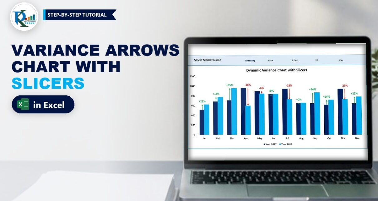
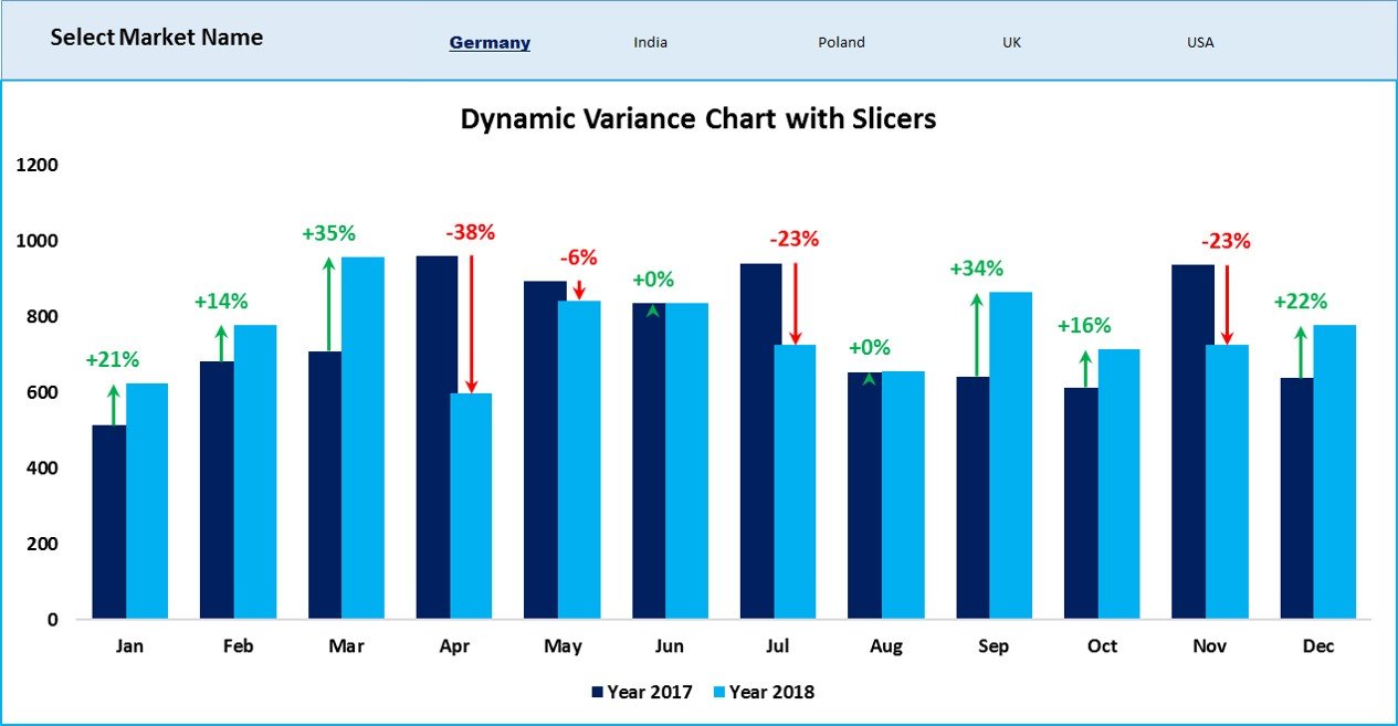
A dynamic variance arrows chart with slicers compares this year with last year month by month, draws a green up arrow or a red down arrow over each pair of columns, and lets you pick the market with a stylish slicer instead of check boxes. Click one market, or hold Ctrl and click several, and the columns, arrows and percentage labels all update. This is Part 2 of PK’s variance chart series: you keep the same chart and helper formulas, feed them from a pivot table, connect a Market Name slicer and give it a custom slicer style.
Watch the Video Tutorial
PK replaces the check boxes from Part 1 with a pivot table and a Market Name slicer, then designs a custom slicer style that blends into the dashboard.
What You Will Build
- A pivot table that totals sales by month and year for whatever market is selected.
- VLOOKUP links that pull those totals into the Support sheet that drives the chart.
- A Market Name slicer laid out in one row of five buttons, without a header.
- A custom slicer style with a matching background, a bold underlined selected item and no white boxes.
- The same variance arrows and percentage labels as Part 1, now in navy and light blue.
Before You Start: The Check Box Version
This tutorial builds on the dynamic variance arrows chart with check boxes. That post walks through the chart in detail: the error-bar arrows, the secondary axis and the Value From Cells labels. The Support sheet here uses the same columns and formulas, so here is a quick recap:
| Column | Header | Formula in row 2 |
|---|---|---|
| A | Month | Jan to Dec |
| B, C | Year 2017, Year 2018 | From the pivot table (Step 3) |
| D | Max Left | =MAX(B2:C2) |
| E | Max Right | =D2 |
| F | Up Error Bar | =IF(C2>B2,C2-B2,NA()) |
| G | Down Error Bar | =IF(C2<B2,B2-C2,NA()) |
| H, I | Up / Down Data Label | TEXT of the change divided by 2017, with a plus or minus sign |
The chart plots A1:E13 as clustered columns, with Max Left and Max Right on the secondary axis, no fill, and custom minus error bars (green begin arrow and red end arrow) whose sizes come from columns F and G. If you have not built it yet, do Part 1 first, then come back.
The Sales Data
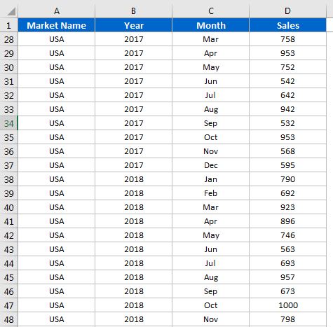
The Data sheet is the same four-column list: Market Name, Year, Month and Sales, with one row for each market, year and month.
Feed the Variance Arrows Chart with Slicers Through a Pivot Table
Step 1: Copy the chart to a new sheet
Insert a new sheet for the slicer version of the dashboard and copy only the chart onto it. The chart still points at the Support sheet, so nothing about the arrows changes.
Step 2: Create the pivot table
On the Support sheet, delete the old 2017 and 2018 formulas in columns B and C. Then select the data on the Data sheet and choose Insert → PivotTable → New Worksheet. In the PivotTable Fields pane:
- Drag Month to Rows.
- Drag Year to Columns.
- Drag Sales to Values (Sum of Sales).
You now have a small grid: months Jan to Dec down column A, the 2017 total in column B and the 2018 total in column C, with a Grand Total on the right. Excel sorts the month names in calendar order because Jan to Dec is a built-in custom list.
Step 3: Pull the totals with VLOOKUP
In Support!B2 enter:
=VLOOKUP(A2,Sheet2!A:C,2,0)and in Support!C2:
=VLOOKUP(A2,Sheet2!A:C,3,0)Fill both down to row 13. Here Sheet2 is the sheet that holds the pivot table; use your own sheet name if it is different.
How the formula works
A2is the month on the Support sheet, for example Jan.Sheet2!A:Cis the pivot table area: month labels in column A, 2017 in column B and 2018 in column C.- The column number
2returns the 2017 total and3returns the 2018 total. - The last argument
0forces an exact match, so Jan only ever matches Jan.
Because the pivot table is filtered by the slicer, these two columns always hold the totals for the selected markets, and every helper column and the chart follow automatically. In PK’s finished file the same pivot table sits on the Support sheet itself, to the right of the helper columns.
Add and Style the Market Slicer
Step 4: Insert the Market Name slicer
Click inside the pivot table, go to PivotTable Analyze (called Analyze or Options in older versions) and choose Insert Slicer. Tick Market Name and click OK. Cut the slicer with Ctrl+X and paste it on the dashboard sheet above the chart.
Step 5: Lay the buttons out in one row
Select the slicer and on the Slicer → Options tab set Columns to 5, so Germany, India, Poland, UK and US sit in a single row. Turn off gridlines on the dashboard sheet with View → Gridlines.
Step 6: Hide the slicer header
Right-click the slicer, choose Slicer Settings and untick Display header. A rectangle with your own caption works better here. Insert a rectangle shape, stretch it across the top of the chart, right-click and choose Send to Back, and give it a light fill colour.
Step 7: Create a custom slicer style
With the slicer selected, open the Slicer Styles gallery, click the More arrow and choose New Slicer Style. Format three elements:
- Whole Slicer: Format → Fill, the same light colour as the rectangle, so the slicer disappears into the banner.
- Selected Item with Data: Format → Font, bold, a dark blue colour, size 12 and a strong font such as Arial Black. PK also adds a single underline so the selected market stands out.
- Unselected Item with Data: leave the font as it is.
Click OK, then open the Slicer Styles gallery again and pick your new style from the Custom group.
Step 8: Remove the white button boxes
The buttons still show a white background. Right-click your custom style in the gallery and choose Modify. Give Selected Item with Data and Unselected Item with Data the same fill colour as the rectangle and click OK. Now the slicer looks like plain text links: the selected market is bold and underlined, the rest are regular.
Step 9: Test it
Click India, then Poland. To compare two or more markets together, hold Ctrl and click each one. The pivot table filters, the VLOOKUPs pick up the new totals, and the arrows and percentages redraw.
Why Use a Slicer Instead of Check Boxes?
PK shows the big benefit at the end of the video. In the Data sheet he renames US to USA, then clicks Data → Refresh All. The slicer button changes to USA on its own, and the chart keeps working.
- No formula edits for new markets. With check boxes, each market needs its own box, cell link and IF block. With a slicer, a new market becomes a new button after a refresh.
- Shorter formulas. Two VLOOKUPs replace the long SUMIFS formula from Part 1.
- Multi-select is built in with Ctrl+Click, and the filter icon on the slicer clears the selection.
The trade-off: a pivot table does not update by itself when the data changes, so remember to refresh.
Modern Excel Alternative
This section is an addition and is not shown in the video. If your data is formatted as an Excel Table (Ctrl+T), you can connect a slicer to the table directly in Excel 2013 and later. The slicer then hides rows instead of filtering a pivot table, and you can total only the visible rows with SUBTOTAL or AGGREGATE. The pivot table method used in the video is simpler for monthly totals and works in Excel 2010, so it is still the recommended route here.
Common Errors and Fixes
The VLOOKUP returns #N/A for some months
The selected market has no rows for that month, so the month is missing from the pivot table. Wrap the formula in IFERROR(…,0), or set the Month field to show items with no data in the pivot’s Field Settings.
The 2017 and 2018 columns are swapped
The VLOOKUP column numbers assume 2017 is the first year column in the pivot table. If you add more years, check the pivot layout and update the column number.
The chart does not change when I click the slicer
The slicer must be connected to the pivot table that the VLOOKUPs read. Right-click the slicer, choose Report Connections and make sure that pivot table is ticked.
Tips
- Use Data → Refresh All after any change to the source data.
- Save your slicer style once and reuse it in every dashboard. The guide on custom slicer styles in Excel shows how to set one as the default.
- Hide the pivot table and the Support sheet once everything works, so users only see the slicer and the chart.
- Microsoft’s article Use slicers to filter data covers every slicer setting used here.
Want It Ready-Made?
If you want the finished workbook with the pivot table, slicer style and chart already set up, get the Dynamic Variance Arrows Chart with Slicers template on NextGenTemplates.com, or browse more Excel templates. To master pivot tables, slicers and dashboards step by step, see the course Excel Pivot Tables and Dashboards.
Related Tutorials
- Dynamic Variance Arrows Chart with Check Boxes (Part 1)
- Custom Slicer Style in Excel: Create, Reuse and Set as Default
- Stylish Pivot Chart with Slicer in Excel
- Dynamic Sales Funnel Chart with Slicers
- Dynamic Chart with Slicer for Employee Count by Age Group
Frequently Asked Questions
How do I select more than one market in a slicer?
Hold Ctrl and click each market. In newer versions you can also turn on the Multi-Select button at the top of the slicer.
Can a slicer control a normal chart that is not a pivot chart?
Yes. The slicer filters a pivot table, helper formulas read the pivot table, and the normal chart plots the helper cells. That lets you use error bars and other formatting that pivot charts do not allow.
Why does the chart not show new data?
Pivot tables only update when you refresh them. Use Data, Refresh All after you change or add data.
How do I hide the slicer header?
Right-click the slicer, open Slicer Settings and untick Display header.
What is the difference between this chart and the check box version?
The chart and arrows are the same. The check box version sums the ticked markets with SUMIFS, while this version filters a pivot table with a slicer and reads it with VLOOKUP.
About the Author
PK is a Microsoft Excel expert and trainer and the founder of PK: An Excel Expert and NextGenTemplates.com. He has been teaching Excel, Power Query and Power BI since 2016 on his YouTube channel.
Conclusion
A dynamic variance arrows chart with slicers keeps everything you liked about the check box version, the arrows, the percentages and the year-on-year columns, and adds a cleaner way to choose markets. A pivot table does the filtering, two VLOOKUPs feed the Support sheet, and a custom slicer style makes the selector look like part of the design. Build it once, refresh when the data changes, and your dashboard is ready for any market you add.