Excel Conditional Formatting Rules Manager: Manage and Clear

Part of the free Module 7: Conditional Formatting · Lesson 12 of 15 · Full Excel course

Updated on 5 September 2026 · Works in Excel 365, 2021, 2019 and 2016 unless noted.

The Conditional Formatting Rules Manager in Excel is the single dialog that lists every conditional formatting rule on a selection, a worksheet, a Table or a PivotTable, so you can create, edit, duplicate, reorder, retarget or delete any of them. Clear Rules is the partner command that strips conditional formatting from selected cells, a whole sheet, a Table or a PivotTable in one click.

Why you need the Rules Manager

Applying a rule takes five seconds. Living with fifty of them is the hard part. Every time you copy a formatted cell, insert rows, drag a fill handle or paste from another sheet, Excel can quietly create another copy of a rule with a slightly different Applies to range. After a few months a working file can carry dozens of overlapping fragments that recalculate on every keystroke and produce colours nobody can explain.

The Rules Manager is the only place that shows you the whole picture: which rules exist, what format each one applies, which cells each one covers and in what order Excel evaluates them. It has looked and behaved the same way from Excel 2007 through Microsoft 365, so the steps below apply to every modern version.

Open the Conditional Formatting Rules Manager

1. Select the range whose rules you want to review. If you want to see every rule on the sheet instead, any single cell will do.
2. Go to Home > Styles > Conditional Formatting > Manage Rules. The legacy key sequence Alt, O, D opens the same dialog; more of these are listed in the Excel shortcut keys course.

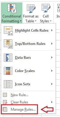
The dialog is modeless, which means you can click cells on the worksheet while it stays open. Use that to check a range before you change it. Changes you make inside the manager are committed when you click Apply (which keeps the dialog open) or OK. Close abandons edits you have not applied.

What each part of the dialog does

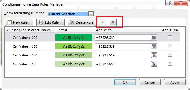
Each row in the list is one rule. The Rule (applied in order shown) column describes the condition, Format shows a live preview of the fill, font and border, Applies to gives the range and Stop If True is a tick box.

Control	What it does	Notes
New Rule	Opens the New Formatting Rule dialog to add a rule to the current Applies to range	Same dialog as Conditional Formatting > New Rule
Edit Rule	Reopens the selected rule so you can change the condition, the formula or the format	Double-clicking the rule row does the same
Delete Rule	Removes the selected rule from the workbook	Only that rule; other rules on the same cells stay
Duplicate Rule	Makes a copy of the selected rule that you can then edit	Present in Microsoft 365 and Excel 2019 and later; not in Excel 2016
Move Up / Move Down	Changes the position of the rule in the evaluation order	Higher rules are evaluated first
Applies to box	Sets the range the rule covers	Editable in place, with a collapse button
Stop If True	Stops Excel evaluating lower rules for cells this rule matches	Covered in depth in the precedence lesson

If your Rules Manager has no Duplicate Rule button, you are on an older build. Copy a rule by selecting a formatted cell, copying it, then using Paste Special > Formats on the target range, or simply rebuild the rule with New Rule.

Show formatting rules for: choosing the scope

By default the manager only lists rules that touch the cells you had selected, which is why it so often looks empty. Open the Show formatting rules for drop-down at the top left and change the scope.

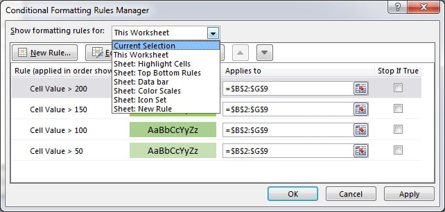
Scope	Lists	When to use it
Current Selection	Only rules that overlap the cells selected when you opened the dialog	Fixing the colours on one block of data
This Worksheet	Every rule on the active sheet, in evaluation order	Auditing, finding forgotten rules, cleaning duplicates
Other sheet names	Every rule on that sheet, without leaving the dialog	Comparing a template sheet with a working copy
This Table	Rules on the Excel Table containing the active cell	Appears only when the selection is inside a Table
This PivotTable	Rules on the PivotTable containing the active cell	Appears only when the selection is inside a PivotTable

Set the scope to This Worksheet whenever a workbook feels slow or a colour appears where you did not expect one. It is the fastest audit in Excel.

Change the range a rule applies to

The Applies to box is editable directly in the list. Click into it, type a new reference such as =$B$2:$G$20, and press Enter. To pick the range on the sheet instead, click the small collapse button at the right of the box: the dialog shrinks to a single line, you drag over the cells, then click the same button again to restore the dialog.

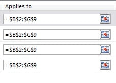
Three things are worth knowing. You can enter several areas separated by commas, for example =$B$2:$B$20,$E$2:$E$20, so one rule can cover columns that are not next to each other. You can point the box at an entire Table column with a structured reference by selecting it with the mouse. And when you widen the range of a formula rule, check the formula still makes sense: the formula is written for the top-left cell of the Applies to range and Excel copies it across the rest like a fill, so =$D2<TODAY() tests column D of each row (whole-row highlight), D$2 would lock the row instead, and =$D$2 locks both and tests one fixed cell. Excel treats the result as TRUE or FALSE, and any non-zero number counts as TRUE. Press F2 before using the arrow keys inside a rule formula box, otherwise the arrows insert cell references instead of moving the cursor.

Rule order in one minute

Rules are evaluated from the top of the list down. When two rules set the same property on the same cell, for example both set a fill colour, the higher rule wins. When they set different properties, for example one sets the fill and another sets the font colour, both apply and the cell shows a combination. Move Up and Move Down change that order, and the change takes effect as soon as you click Apply.

Stop If True and the finer points of precedence, including why data bars and icon sets need it, are covered fully in Conditional formatting rule precedence and Stop If True.

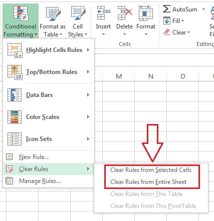
Clear Rules from cells, sheets, Tables and PivotTables

1. Select the cells you want to clean, or click any single cell if you intend to clear the whole sheet.
2. Go to Home > Styles > Conditional Formatting > Clear Rules.
3. Choose the scope you need from the submenu.

Command	Effect	Available when
Clear Rules from Selected Cells	Removes conditional formatting from the selection only. A rule that also covers cells outside the selection survives, with a smaller Applies to range	Always
Clear Rules from Entire Sheet	Deletes every conditional formatting rule on the active sheet	Always
Clear Rules from This Table	Removes rules from the Excel Table that contains the active cell	Active cell is inside a Table
Clear Rules from This PivotTable	Removes rules from the PivotTable that contains the active cell	Active cell is inside a PivotTable

Clear Rules is a formatting command, not a data command. It leaves values, formulas and manual fill colours untouched. Ctrl+Z undoes it, but only until you save and close the file, so on a shared workbook prefer deleting individual rules in the manager.

Find every cell that has conditional formatting

The Rules Manager tells you which ranges are covered. To see the cells themselves highlighted on the sheet, use Go To Special.

1. Click any cell on the sheet.
2. Go to Home > Editing > Find & Select > Conditional Formatting. Excel immediately selects every cell on the sheet that carries a rule.
3. For finer control, press F5 (or Ctrl+G), click Special, choose Conditional formats, then pick All or Same. All selects every conditionally formatted cell on the sheet. Same selects only the cells that carry the same conditional format as the active cell, which is how you find the true extent of one rule.
4. With the cells selected, look at the status bar count, or apply a temporary manual fill to see the shape of the selection before you decide what to clear.

Data Validation sits in the same Go To Special dialog with the same All and Same choices, so the technique transfers straight to the Data Validation course.

Tidy fragmented rules created by copy and paste

Rule fragmentation is the most common cause of a slow, colourful mess. Inserting rows, copying a formatted cell to a new row, or pasting a block from another sheet all split one clean rule into several near-identical rules with ranges such as =$B$2:$B$9, =$B$10, =$B$11:$B$14. Fix it like this.

1. Open Manage Rules and set the scope to This Worksheet.
2. Identify the duplicates: identical rule descriptions with identical format previews.
3. Keep one of them. Click its Applies to box and type the full, correct range, for example =$B$2:$G$500.
4. Select each leftover duplicate and click Delete Rule.
5. Click Apply, check the sheet still looks right, then OK.

To stop it happening again, convert the data to an Excel Table with Ctrl+T. A rule applied to a Table column grows with the Table automatically when rows are added, so no new fragments are created. Copying rules deliberately, and managing them across sheets and Tables, is covered in copy, paste and manage conditional formatting across sheets and Tables.

Worked example: cleaning up a sales sheet

A sales sheet has been edited by three people. Column D holds the value and column F the status.

Row	Order	Value (D)	Status (F)
2	SO-1001	1,920	Open
3	SO-1002	480	Closed
4	SO-1003	2,310	Open
5	SO-1004	750	Hold

1. Click any cell, open Home > Conditional Formatting > Manage Rules and set the drop-down to This Worksheet. Six rules appear: three identical Cell Value greater than 1000 rules on =$D$2, =$D$3:$D$4 and =$D$5, plus a Specific Text rule for Open, a leftover data bar and a stray rule pointing at =$D$50.
2. Select the first greater than rule, click its Applies to box and type =$D$2:$D$500. Press Enter.
3. Select the second and third greater than rules and click Delete Rule for each. Delete the rule pointing at =$D$50 as well.
4. Select the leftover data bar rule and click Delete Rule, since column D already has a colour rule.
5. Select the Specific Text rule for Open, click Move Up so it sits above the value rule, then click Apply.
6. Close the dialog and press F5 > Special > Conditional formats > All to confirm only D2:D500 and F2:F500 are selected.

Result: three rules instead of six, one clean Applies to range per rule, and no stray formatting below row 5.

Tips and common mistakes

• Painting over a colour does not remove the rule. A manual fill sits underneath the conditional format and the rule wins. Use Clear Rules or Delete Rule.
• The manager opens on Current Selection. An empty list almost always means the wrong scope, not the absence of rules. Switch to This Worksheet first.
• Delete the rule, not the row. Deleting rows to remove formatting destroys data and usually leaves the rule behind with a shifted range.
• Avoid whole-column Applies to ranges. =$D:$D makes Excel evaluate a million cells. Use a generous but finite range or an Excel Table.
• Check Applies to after inserting rows. Rows inserted inside the range extend the rule; rows added below it do not.
• Apply before you judge. Nothing changes on the sheet until you click Apply or OK, so a reordering that looks wrong may simply not be committed yet.
• Conditional formats survive Clear Contents. They are removed by Home > Clear > Clear Formats or Clear All.

Errors and how to fix them

Symptom	Cause	Fix
Rules Manager list is empty although cells are coloured	Scope is Current Selection and the selection misses the rule, or the colour is a manual fill	Set Show formatting rules for to This Worksheet; if it is still empty the fill is manual
The same rule is listed many times	Fragmentation from copy, paste or inserted rows	Widen one rule’s Applies to range and delete the duplicates
Workbook is slow to scroll and type in	Whole-column ranges, volatile functions or dozens of overlapping rules	Trim Applies to ranges, remove duplicates, convert the data to a Table
A colour does not appear even though the condition is met	A higher rule sets the same property, or Stop If True is ticked above it	Use Move Up, or clear the Stop If True tick on the higher rule
Clear Rules from Selected Cells left some colour behind	Another rule covers those cells from a wider range	Open the manager on This Worksheet and delete the wider rule
No Duplicate Rule button	Excel 2016 or earlier	Copy a formatted cell and use Paste Special > Formats, or rebuild with New Rule
Formatting disappears after a PivotTable refresh	The rule was scoped to selected cells rather than to the field	Reapply and choose the field-based option in the Formatting Options button

Practice exercise

Open the course practice file or any sheet of your own, then:

1. Apply a Greater Than rule to B2:B9, then copy B2 to B12 and open Manage Rules on This Worksheet. Count how many rules now exist.
2. Merge them back into one by editing the Applies to box to =$B$2:$B$12 and deleting the duplicate.
3. Add a second rule with a different font colour, then use Move Up and Move Down and note which colour wins each time.
4. Use Find & Select > Conditional Formatting to select every formatted cell, then repeat with F5 > Special > Conditional formats > Same and compare the selections.
5. Clear the rules from B2:B5 only, then reopen the manager and check what happened to the Applies to range of the surviving rule.

Key takeaways

• Home > Conditional Formatting > Manage Rules opens the Conditional Formatting Rules Manager, a modeless dialog you can use with the sheet still visible.
• Show formatting rules for controls the scope: Current Selection, This Worksheet, another sheet, This Table or This PivotTable.
• New, Edit, Delete and Move Up or Move Down are on every version; Duplicate Rule is in Microsoft 365 and Excel 2019 and later.
• The Applies to box is editable in place, accepts several comma separated areas and has a collapse button for picking the range on the sheet.
• Clear Rules works on selected cells, the entire sheet, this Table or this PivotTable, and removes formatting without touching data.
• Find & Select > Conditional Formatting, or Go To Special with All versus Same, shows exactly which cells a rule reaches.
• Merging fragmented ranges and deleting duplicate rules is the quickest fix for a slow, over-coloured workbook.

Related lessons

• Conditional Formatting course hub
• Conditional formatting with a formula: rows and columns
• Rule precedence and Stop If True
• Copy, paste and manage conditional formatting across sheets and Tables
• Highlight Cells Rules: all 7 presets
• Refresh a PivotTable and change its source
• Microsoft Support: Manage conditional formatting rule precedence

Frequently asked questions

Where is the Conditional Formatting Rules Manager in Excel?

Select a cell, then choose Home > Styles > Conditional Formatting > Manage Rules. The legacy key sequence Alt, O, D opens the same dialog. If the list looks empty, change the Show formatting rules for drop-down from Current Selection to This Worksheet, because by default the manager only shows rules that touch the cells you had selected.

How do I see every conditional formatting rule in a workbook?

There is no single workbook view. Open the Rules Manager and use the Show formatting rules for drop-down, which lists every sheet by name, so you can step through them one at a time without leaving the dialog. On each sheet you can also press F5, click Special and choose Conditional formats with All to select the affected cells.

What is the difference between Delete Rule and Clear Rules?

Delete Rule removes one specific rule from the workbook, wherever it applies. Clear Rules removes all conditional formatting from a scope you choose: the selected cells, the entire sheet, this Table or this PivotTable. Use Delete Rule for surgery and Clear Rules when you want a clean slate on a block of cells.

Why does my conditional formatting split into many rules?

Copying formatted cells, inserting rows and pasting blocks from other sheets all duplicate the rule with a new Applies to range. Fix it by widening one rule’s Applies to range in the manager and deleting the duplicates. Converting the data to an Excel Table with Ctrl+T prevents most future fragmentation, because the range grows with the Table.

Does every version of Excel have the Duplicate Rule button?

No. Duplicate Rule is available in Microsoft 365 and Excel 2019 and later. In Excel 2016 the manager offers only New Rule, Edit Rule and Delete Rule. On those versions, copy a formatted cell and use Paste Special > Formats on the target range, or rebuild the rule with New Rule and change the one setting you need.

Want the finished version? Ready-made Excel KPI dashboards with clean, tuned conditional formatting already built in are available at NextGenTemplates.com.