The function in Excel is used to lookup and retrieve data from a specific column in a table. It’s an extremely useful function when working with large data sets and is commonly used to combine data from multiple tables.
The basic syntax of the VLOOKUP function is as follows:
=VLOOKUP(lookup_value, table_array, col_index_num, [range_lookup])
lookup_value: Select the value that you want to search. It can be a number, text, or a reference to a cell that contains the value.
- table_array: The range of cells that make up the table. It should include the lookup value and the data that you want to retrieve.
col_index_num: The number of the column in the table that you want to return the value from. For the first column, take 1, and for the second column take 2, and so on.
[range_lookup]: This is an optional argument. If it is set to TRUE or omitted, the function will use an approximate match. This means that it will find the closest match to the lookup value and return the corresponding value. If it is set to FALSE, the function will use an exact match.
Here is an example of how the VLOOKUP function could be used:
=VLOOKUP(A2,B2:D8,2,FALSE)
This formula looks up the value in cell A2 in table B2:D8 and returns the value from the second column of that table. The range_lookup is set to false which means the function will use an exact match for the lookup value.
Note that this is a basic example, the function can be used in many ways, with multiple tables, and even in combination with other functions.
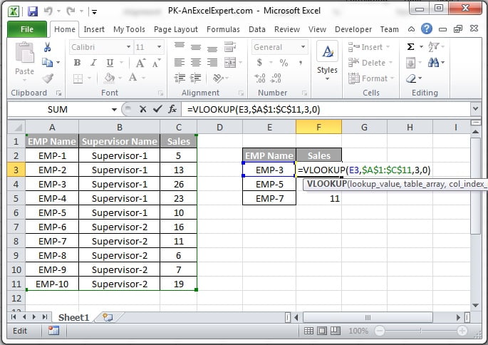
Another example is given in below screenshot
Also learn below useful functions:
- 6 Powerful Dynamic Array Function in Excel
- 6 Powerful Dynamic Array Function in Excel
- INDEX Formula
- HLOOKUP-formula
- VLOOKUP by cell background color