Quality Check List in Excel with Pass/Fail Icons (Free Template)

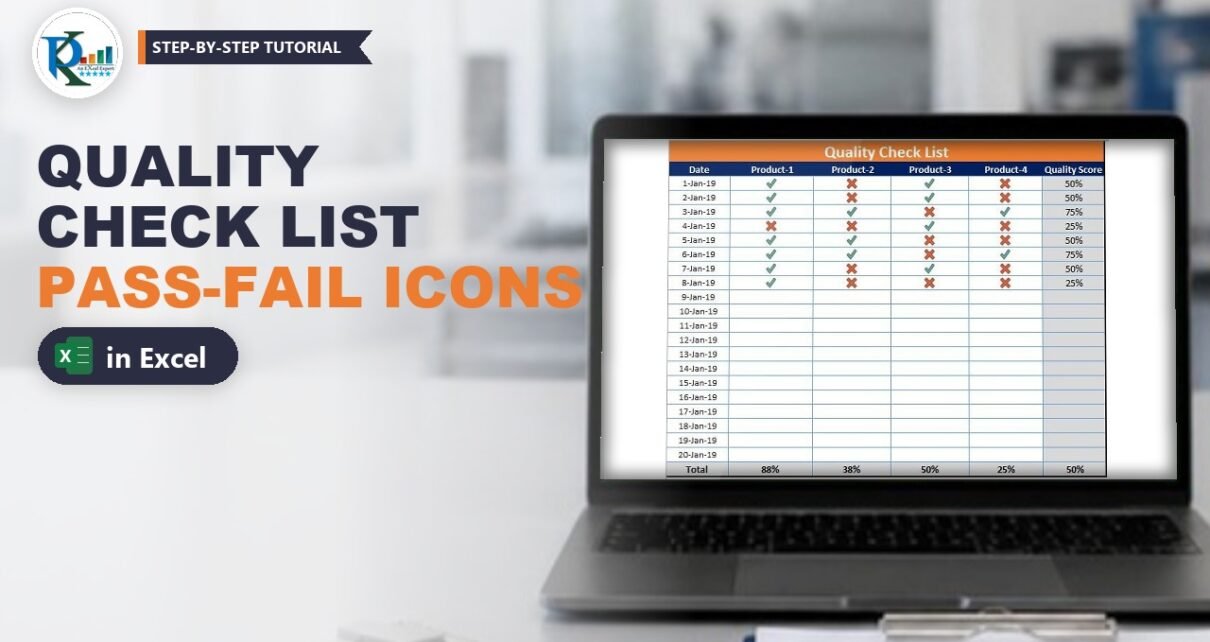
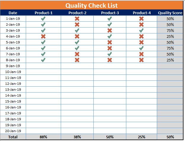
This quality check list in Excel lets your quality team mark every product as Pass or Fail from a drop-down, and Excel turns each choice into a green tick or a red cross. A quality score for every day, every product and the whole period updates by itself. Behind the icons there is no VBA, only three classic tools: a custom number format, a data validation list and an icon set in conditional formatting. You can use the same idea for Yes/No, Pending/Completed or any to-do list.

⬇️  Download the Quality Check List
.xlsx workbook (13 KB) · Excel 2010 and later · no macros

Watch the Video Tutorial

In the video, PK builds the check list on a new sheet: the table and formatting, the Pass/Fail custom format, the drop-down, the icon set and finally the AVERAGE formulas for the quality score.

What You Will Build

• A dated check list table with one column per product (Product-1 to Product-4).
• A Pass/Fail drop-down in every check cell, which really stores 1 or 0.
• Icons instead of text: a green tick for Pass and a red cross for Fail.
• A Quality Score per day, per product and overall, shown as a percentage.
• No VBA: the file is a normal .xlsx workbook.

How the Workbook Is Laid Out

The download has two sheets. Quality Check List is the finished template with 20 dates. Sheet1 is the version PK builds in the video with 15 dates, so you can compare your own work with it.

• A1:F1: the merged title.
• Row 2: headers Date, Product-1 to Product-4 and Quality Score.
• A3:A22: the dates (1-Jan-19 to 20-Jan-19), with Total in A23.
• B3:E22: the Pass/Fail cells.
• F3:F22 and row 23: the score formulas.
• I1:I2: two support cells, 1 and 0, that feed the drop-down.

Part 1: Build the Check List Table

Step 1: Create the headers and dates

Type Date in A2, your product names in B2:E2 and Quality Score in F2. Add your dates below (the template uses one row per day) and type Total in the row under the last date. You can add more products: insert the new columns between two existing product columns, so every formula range grows with them.

Step 2: Format the table

• Turn off gridlines with View > Gridlines.
• Select A1:F1, click Merge & Center and type the title. The template uses an orange fill with a white, bold, bigger font.
• Give the header row a dark blue fill with a white bold font, and the Total row and Quality Score column a grey fill with bold text.
• Select the table, press Alt, O, E (or Ctrl + 1) to open Format Cells, and on the Border tab pick a colour and click Outline and Inside.

Part 2: Show 1 and 0 as Pass and Fail

Step 3: Add the support cells

Away from the table, type 1 in I1 and 0 in I2. These two numbers are the real values behind Pass and Fail. Storing numbers, not text, is what lets you average them later.

Step 4: Apply the custom number format

Select I1:I2, open Format Cells > Number > Custom and type this in the Type box:

"Pass";;"Fail"

Click OK. I1 now shows Pass and I2 shows Fail, while the formula bar still shows 1 and 0. Apply exactly the same custom format to the check cells B3:E22.

How the custom format works

• A custom number format can have four sections separated by semicolons: positive; negative; zero; text.
• "Pass" is the positive section, so any number above zero is displayed as Pass.
• The negative section is left empty, because you never enter negative numbers here.
• "Fail" is the zero section, so 0 is displayed as Fail.

As PK shows in the video, typing 5 also displays Pass, because every positive number uses the first section. The drop-down in the next step makes sure only 1 or 0 is entered.

Part 3: Create the Pass/Fail Drop-Down

Step 5: Add a data validation list

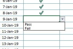
Select B3:E22 and open Data > Data Validation (shortcut Alt, D, L). In Allow choose List, and in Source select the support cells:

=$I$1:$I$2

Click OK. Every check cell now has a drop-down with Pass and Fail. Because the list shows the formatted values of I1:I2, you see the words, but the cell receives the number 1 or 0. You can confirm it in the formula bar.

Part 4: Turn Pass and Fail into Icons

Step 6: Add an icon set rule

Select B3:E22 again and go to Home > Conditional Formatting > New Rule. Keep Format all cells based on their values, set Format Style to Icon Sets and pick the tick, exclamation mark and cross symbols. Then set the rules exactly like this:

• Icon 1: green tick when value is > 0, Type Number.
• Icon 2: change it to the red cross, when value is >= 0, Type Number.
• Icon 3: leave the red cross for values below 0.

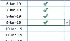
Click OK. A Pass (1) now gets a tick and a Fail (0) gets a cross, but the words are still visible next to the icons.

Step 7: Show the icon only

Open the rules manager with Home > Conditional Formatting > Manage Rules (shortcut Alt, O, D), select the Icon Set rule, click Edit Rule and tick Show Icon Only. Now the check cells show just the tick or the cross. Empty cells show nothing, so you can see at a glance which checks are still open.

Part 5: Calculate the Quality Score

Step 8: Score for each day

In F3 enter the formula below, format it as a percentage and fill it down to F22:

=IFERROR(AVERAGE(B3:E3),"")

Step 9: Score for each product and overall

In B23 enter the formula and copy it across to E23. In F23 average the whole check range:

B23: =IFERROR(AVERAGE(B3:B22),"")
F23: =IFERROR(AVERAGE(B3:E22),"")

Format row 23 as a percentage too. If Excel shows a green error triangle on F23 (because its formula differs from the cells around it), select the cell and choose Ignore Error.

How the formula works

• Every Pass is 1 and every Fail is 0, so the average of a range is simply the share of passes. One pass and one fail give 50%; two passes and one fail give 67%.
• AVERAGE ignores empty cells, so products that have not been checked yet do not pull the score down.
• When a whole row is empty, AVERAGE returns #DIV/0!. IFERROR(...,"") catches that error and shows a blank cell instead.

Count Passes and Fails (Addition)

This is not in the original file or video. If you also want counts, use COUNTIF on the stored numbers, not on the words, because the cells really hold 1 and 0:

Passes: =COUNTIF(B3:E22,1)
Fails:  =COUNTIF(B3:E22,0)

In Microsoft 365 you can also build a check list with the new in-cell checkboxes (Insert > Checkbox), which store TRUE or FALSE. The Pass/Fail format above has the advantage of working in every Excel version from 2010 onward.

Common Errors and Fixes

The drop-down shows 1 and 0 instead of Pass and Fail

The custom format is missing on I1:I2. Apply "Pass";;"Fail" to the support cells, not only to the check cells.

Pass and Fail text still shows next to the icons

Show Icon Only is not ticked. Open Manage Rules (Alt, O, D), edit the Icon Set rule and tick Show Icon Only, as in Step 7.

The Quality Score shows Pass or Fail

The score cell inherited the custom format. Change it to Percentage, as PK does in the video.

A cell shows Pass but the score looks wrong

Every positive number uses the first section of the custom format, so a 5 also displays as Pass and pushes the average above 100%. This usually happens when values are pasted into the range, because pasting bypasses data validation. Check the formula bar and pick 1 or 0 from the drop-down instead.

Tips

• Change the words in the custom format to "Yes";;"No" or "Completed";;"Pending" for other kinds of lists.
• Hide column I or move the support cells to another sheet once everything works, so nobody overwrites them.
• Protect the sheet and unlock only B3:E22, so users can tick checks without breaking the formulas.
• To add dates, insert rows inside the date range (for example above the last date), so the AVERAGE ranges, validation and icon rule grow automatically. Rows inserted directly above Total sit outside the ranges.
• Microsoft explains each section of a format code in its guide to customizing a number format.

Want It Ready-Made?

If you need a full quality tracking system with defect logging and reports, the Quality Control Tracker in Excel on NextGenTemplates.com is ready to use, and you can browse more quality control templates for Excel.

Related Tutorials

• Icon Sets in Excel: Traffic Lights, Thresholds and Custom Icons
• Drop-Down List in Excel with Data Validation
• Arrow Symbols with Custom Formatting in Excel
• Quality Control Check List Template in Excel
• Conditional Formatting in Excel: Full Course

Frequently Asked Questions

Does this quality check list use VBA?

No. It uses a custom number format, a data validation list, an icon set and AVERAGE formulas, so it works in a normal .xlsx file without macros.

Why does the drop-down store 1 and 0 instead of the words?

Numbers can be averaged into a quality score and can drive an icon set. The custom number format only changes how 1 and 0 are displayed, so you see Pass and Fail while Excel calculates with numbers.

How is the Quality Score calculated?

It is the AVERAGE of the 1 and 0 values in the row, column or whole range, shown as a percentage. Empty cells are ignored, and IFERROR shows a blank when nothing is checked yet.

Can I use Yes and No instead of Pass and Fail?

Yes. Change the words in the custom number format of the support cells and the check cells, as explained in Step 4. The drop-down, icons and score keep working.

Can I add more products or dates?

Yes. Insert new columns between two existing products and new rows inside the date range, so the formulas, validation and icon rule expand with the table.

About the Author

PK is a Microsoft Excel expert and trainer and the founder of PK: An Excel Expert and NextGenTemplates.com. He has been teaching Excel, VBA, Power Query and Power BI since 2016 on his YouTube channel.

Conclusion

A quality check list in Excel does not need macros to look professional. Store 1 and 0, display them as Pass and Fail with a custom number format, pick them from a drop-down, swap them for icons with conditional formatting, and let AVERAGE turn them into a quality score. Download the template, change the product names and dates, and your team can start checking today.