Zonal Dashboard in Excel: Form Controls and Free File

Part of the free Module 11: Excel Dashboards · Lesson 6 of 10 · Full Excel course

Updated on 5 September 2026 · Works in Excel 365, 2021, 2019 and 2016 unless noted.

The Zonal Dashboard in Excel shows regional KPIs for four zones and three metrics on one page. Option buttons switch the zone, a combo box picks the month and three checkboxes show or hide each metric on a monthly trend chart. It is a free download built with Form Controls, INDEX and SUMIFS, and no macros. This lesson explains how the controls drive the cards and the chart, and how to load your own zones and numbers.

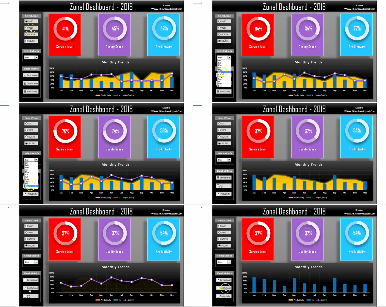
What the Zonal Dashboard shows

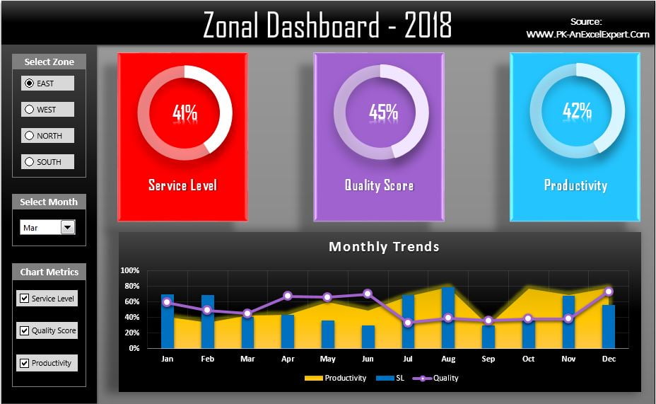
The top band holds the selected zone’s three metrics for the chosen month in three KPI cards. The zone is chosen with four option buttons (North, South, East and West in the sample) and the month from a combo box. The lower band is a twelve-month trend chart for the selected zone, and three checkboxes let the reader switch each metric line on or off. Because zone and month are user controls rather than filters on a PivotTable, the dashboard recalculates instantly, needs no refresh and works from a plain data table.

It is the natural next step after the Quick Dashboard: the same linked-cell idea, but with three kinds of control working together and a chart that can hide series.

The workbook structure

The file has two sheets that matter. The Data sheet holds one row per zone per month with the three metric columns, so four zones and twelve months give 48 rows. The Dashboard sheet holds the controls, three linked cells, a small calculation block, a chart-feed table and the visuals. Keeping the calculation block on the dashboard sheet in hidden columns is fine for a file this size; the larger projects in this course move it to a separate sheet.

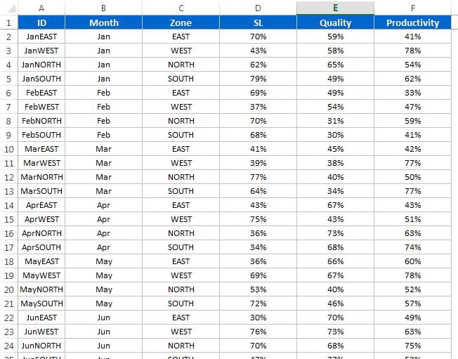
Zonal Dashboard data table in Excel with zone, month and three metric columns — One row per zone per month: the data table behind the Zonal Dashboard

How it is built

Element	Technique	Formula or feature
Zone selector	Four Form Control option buttons	One shared cell link (B2) holding 1 to 4; `=INDEX({"North","South","East","West"}, $B$2)` returns the zone name
Month selector	Form Control combo box	Input range = month list, cell link (B3) holding 1 to 12; `=INDEX(Months, $B$3)` returns the month label
KPI cards	Shapes linked to cells	`=SUMIFS(Data!$D:$D, Data!$A:$A, $C$2, Data!$B:$B, $C$3)` per metric
Metric switches	Three Form Control checkboxes	Cell links holding TRUE or FALSE
Chart-feed table	12 rows by 3 metrics	`=IF($F$2, SUMIFS(Data!$D:$D, Data!$A:$A, $C$2, Data!$B:$B, $A10), NA())`
Trend chart	Line chart with markers	Plots the chart-feed table; #N/A points are not drawn
Chart title	Linked cell	`=$C$2 & " monthly trend"`

Option buttons and the combo box

All four option buttons come from Developer > Insert > Form Controls. Buttons drawn on the same sheet form one group and share a single cell link, which holds 1, 2, 3 or 4. An INDEX formula turns that number into the zone name that the SUMIFS formulas use as a criterion. The combo box works the same way: its input range is the list of twelve month labels and its cell link receives the position of the chosen month. A second INDEX turns the position into the month label.

The KPI cards

Each card is a rounded rectangle. Select the shape, click in the formula bar, type =$H$2 (the cell that holds the metric) and press Enter, and the shape displays whatever that cell shows. The cell itself uses SUMIFS keyed on the selected zone and month. Because every zone and month pair appears exactly once in the data table, SUMIFS simply returns that row’s value; if you later load several rows per pair, it totals them, which is usually what you want.

The chart-feed table and the checkboxes

The trend chart never reads the Data sheet directly. It reads a chart-feed table of twelve rows (months) by three columns (metrics). Each cell holds an IF wrapped around a SUMIFS: if the metric’s checkbox is ticked, return the value; otherwise return NA(). Excel does not plot #N/A on a line chart, so an unticked metric vanishes instead of collapsing to zero. Tick it again and the line reappears. This is the same trick as the dynamic chart with checkboxes lesson.

Worked example

Suppose the Data sheet holds these rows for the North zone (the sample has four zones and twelve months).

Zone	Month	Revenue	Orders	Return rate
North	Jan	42,000	310	3.2%
North	Feb	45,500	335	2.9%
North	Mar	48,200	352	2.6%

Click the North option button: B2 becomes 1 and C2 shows North. Choose Feb in the combo box: B3 becomes 2 and C3 shows Feb. The Revenue card formula =SUMIFS(Data!C:C, Data!A:A, "North", Data!B:B, "Feb") returns 45,500. Untick the Return rate checkbox: its cell link turns FALSE, the third column of the chart-feed table fills with #N/A, and the return-rate line disappears from the trend chart while Revenue and Orders stay.

How to use it with your own data

Download the file below and open the Data sheet.
Replace the zone names, month labels and metric values, keeping one row per zone per month.
Rename the four option buttons and three checkboxes to match your zones and metrics: right-click the control and choose Edit Text.
If you have more than four zones, draw extra option buttons on the same sheet (they join the group and share the cell link) and extend the zone list that INDEX reads.
If you have more than twelve months, extend the combo box input range under Format Control and add rows to the chart-feed table.
Set the number format on each card cell (currency, whole number, percent) and save.

Download the free file

Click here to download the Zonal Dashboard Excel file. It is a plain .xlsx with no macros.

Watch the video

Two-part build tutorial:

Tips and common mistakes

One cell link for all option buttons. If each button has its own link, two buttons can appear selected and the zone never changes.
Use NA(), not zero, to hide a series. Zero draws a flat line along the axis; #N/A leaves a gap or removes the line entirely.
Match labels exactly. SUMIFS treats “North ” with a trailing space as a different zone. Use TRIM on imported data.
Mind mixed scales. A percentage metric next to revenue is unreadable on one axis. Plot it on a secondary axis or convert it to a comparable scale.
Fix the axis bounds. When the chart rescales every time a metric is hidden, readers lose the reference. Set minimum and maximum manually.
Keep the data as an Excel Table. Press Ctrl+T on the Data sheet so new rows are picked up by the SUMIFS ranges without editing formulas.
Excel 365 alternative. The Insert > Checkbox cell control returns TRUE or FALSE straight in the cell, so you can drop the Form Control checkbox and its link.

Errors and how to fix them

Symptom	Cause	Fix
Cards show zero	Zone or month label in the data does not match what INDEX returns	Check spelling and spaces; compare with `=C2=Data!A2`
Combo box shows #REF!	Input range was moved or deleted	Right-click, Format Control, reset the input range and cell link
Chart shows #N/A in the legend or a blank series	Checkbox unticked, or the chart-feed formula points at the wrong link	Tick the box; confirm each IF reads its own checkbox cell
Two option buttons selected	Buttons have different cell links	Set every button in the group to the same link
Cards stop updating after new rows	SUMIFS ranges end before the new data	Convert the data to a Table or use whole-column references

Practice exercise

Add a fifth zone, Central, with twelve rows of data, a fifth option button and an extended zone list.
Add a fourth metric column and a fourth checkbox, and extend the chart-feed table so the chart can show it.
Replace the combo box with a Data Validation drop-down of month names and use MATCH to return the month number.
Add a fourth card that shows the selected zone’s year-to-date revenue with SUMIFS on months up to the selected one.
Apply a conditional formatting rule that turns the return-rate card red when it exceeds 3 percent.

Key takeaways

Option buttons, combo boxes and checkboxes all write to a linked cell; the formulas do the rest.
SUMIFS keyed on the selected zone and month pulls the card values from a flat data table.
A chart-feed table with IF and NA() lets one chart show or hide any combination of metrics.
Excel skips #N/A on line charts, which is why hidden metrics disappear cleanly.
Keep data, calculation and display separate so the dashboard survives a data refresh.

Related lessons

Frequently asked questions

Do I need the Developer tab to use the Zonal Dashboard?

No. The option buttons, combo box and checkboxes already exist in the download. You need the Developer tab only to add or edit Form Controls. Enable it under File > Options > Customize Ribbon and tick Developer.

Can I use this dashboard for more than four zones?

Yes. Draw extra option buttons on the same sheet so they join the existing group and share the cell link, then extend the zone list that INDEX reads. Add the new zone’s rows to the Data sheet and the SUMIFS formulas pick them up.

Why do the cards show zero after I paste my data?

The zone or month labels in the Data sheet do not match the labels the controls return. Look for extra spaces, different spelling or a month typed as a date rather than text. Correct the labels or wrap the data column in TRIM.

Why does a hidden metric draw a line at zero?

The chart-feed formula returns 0 instead of NA() when the checkbox is unticked. Excel plots zero as a point, but skips #N/A. Change the IF’s false branch to NA() and the line disappears.

Does the Zonal Dashboard work in Excel for the web?

The formulas and chart work, but Form Controls cannot be clicked in a browser. If the file must run online, replace the option buttons and combo box with Data Validation drop-downs and the checkboxes with cells holding TRUE or FALSE.

Want the finished version? Ready-made Excel dashboards, trackers and VBA systems are available at NextGenTemplates.com.