Format Only Cells That Contain in Excel: All 7 Options

Part of the free Module 7: Conditional Formatting · Lesson 7 of 15 · Full Excel course

Updated on 5 September 2026 · Works in Excel 365, 2021, 2019 and 2016 unless noted.

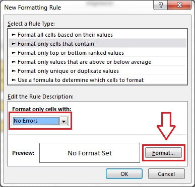
Format only cells that contain is the second rule type in Excel’s New Formatting Rule dialog. It formats a cell when its own content passes one test: a Cell Value comparison, Specific Text, a date occurring in a relative period, Blanks, No Blanks, Errors or No Errors. It is the rule type behind most of the Highlight Cells presets, with more operators and the full Format Cells dialog.

What the rule does and when to use it

This rule tests each cell in the Applies to range against itself. Nothing else in the row or sheet is consulted, which makes it fast and easy to audit. It answers the everyday questions: which figures sit between two limits, which status cells say Pending, which fields are still empty, which formulas have broken.

Compared with the one-click presets under Highlight Cells Rules, this rule type adds three things. It gives you every comparison operator, including greater than or equal to and not between. It adds four tests the presets do not expose at all: Blanks, No Blanks, Errors and No Errors. And it always opens the full Format Cells dialog, so a single rule can set a number format, font style, border and fill together. The behaviour is identical in Excel 2016, 2019, 2021 and Microsoft 365.

The seven options at a glance

Option	Tests	What you enter	Typical use
Cell Value	The underlying number, date or text value	An operator plus one or two values or cell references	Sales between 100 and 200
Specific Text	The characters in the cell	containing, not containing, beginning with or ending with, plus the text	Status containing Pending
Dates Occurring	Real Excel dates against a relative period	A period picked from a list	Deliveries due this week
Blanks	Empty cells	Nothing, just a format	Missing entries on a form
No Blanks	Cells with any content	Nothing, just a format	Shading completed entries
Errors	Cells showing an error value	Nothing, just a format	Flagging broken formulas
No Errors	Cells without an error value	Nothing, just a format	Shading valid results only

Step by step: open the New Formatting Rule dialog

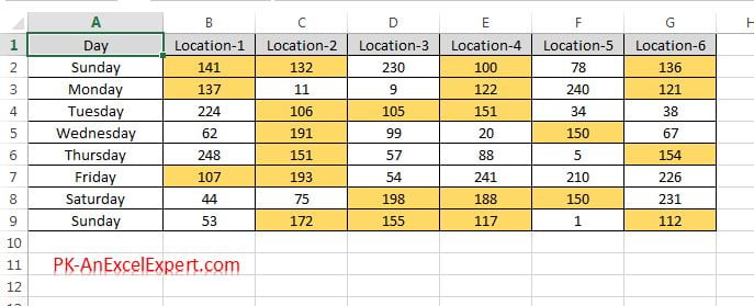
The examples use a day-wise, location-wise sales table in B2:G9.

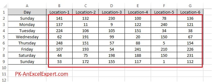
1. Select the range B2:G9. Whatever you select becomes the rule’s Applies to range.
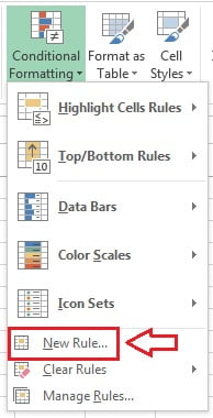
2. Go to Home > Styles > Conditional Formatting > New Rule.

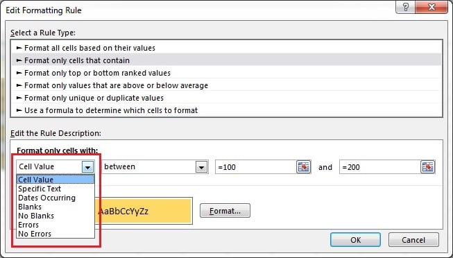
3. Select Format only cells that contain in the rule type list. The first drop-down under Edit the Rule Description holds the seven options.

Cell Value: comparing numbers and dates

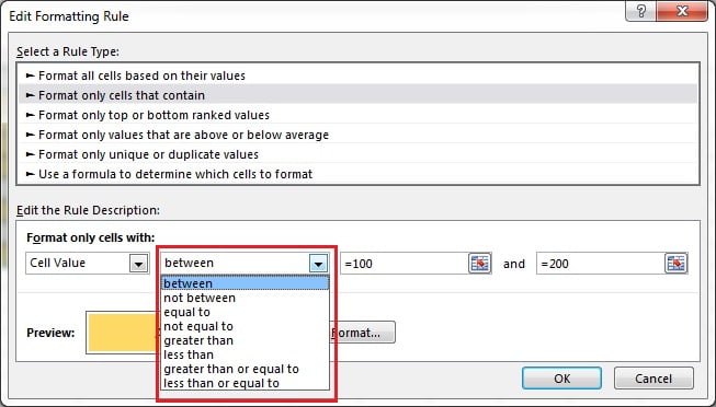
Cell Value compares the value stored in the cell with one limit, or with two when you choose between or not between. To highlight sales between 100 and 200:

1. Keep Cell Value in the first drop-down and choose between in the second.
2. Enter 100 and 200, or click the cells that hold the limits so the thresholds can be changed later without editing the rule.

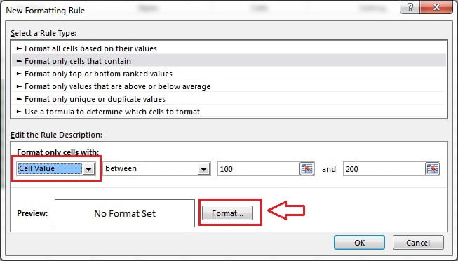
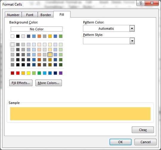
3. Click Format. The Format Cells dialog opens with Number, Font, Border and Fill tabs. Choose a fill colour and click OK.

4. Click OK again to apply the rule. Every value from 100 to 200 inclusive is highlighted.

The operator drop-down offers eight choices: between, not between, equal to, not equal to, greater than, less than, greater than or equal to, and less than or equal to. The last two are the reason most people come to this dialog, because the Highlight Cells presets stop at strict greater than and less than.

Because the value boxes accept references, a rule can be driven by input cells. Type the lower limit in J1 and the upper limit in J2, then enter =$J$1 and =$J$2. The dollar signs lock both references so every cell in B2:G9 is compared with the same two input cells. Leave them relative and Excel shifts the reference for each cell, which almost never gives the result you want.

Specific Text: containing, not containing, beginning with, ending with

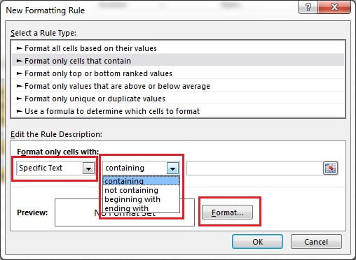
Specific Text looks at the characters displayed in the cell rather than the underlying value. The second drop-down offers four tests: containing, not containing, beginning with and ending with. Type the text in the box or point to a cell that holds it.

Matching is not case-sensitive, so loc matches Location-1 and LOCATION-2. Wildcards are not supported here; the fragment itself does the work of a wildcard. Use containing for status columns and comments, beginning with for product or account codes that share a prefix, and ending with for file extensions or email domains. Pointing at a cell such as =$J$4 turns the rule into a live search box: type a fragment there and the matching cells light up.

Dates Occurring: relative date periods

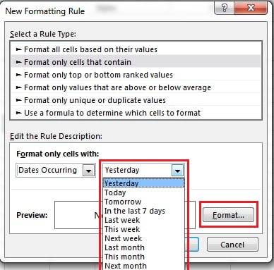
Dates Occurring works only on real Excel dates, never on text that looks like a date. The period list holds ten choices: Yesterday, Today, Tomorrow, In the last 7 days, Last week, This week, Next week, Last month, This month and Next month. Weeks run Sunday to Saturday and the periods follow the system clock, so a due-date column re-highlights itself every morning with no edit to the rule.

The list has no entry for overdue, due in three days, or weekends. Those need a formula rule, which is covered in the dates lesson later in this course.

Blanks and No Blanks

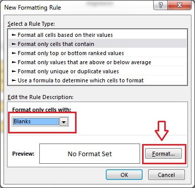
Blanks formats every empty cell in the Applies to range. Excel builds this test as a length check after trimming, so a cell holding only spaces counts as blank, and so does a formula returning an empty string. It is the quickest way to show which fields on a data-entry sheet still need attention, and it needs no criteria at all: pick the option, set a format, click OK.

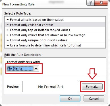
No Blanks is the mirror image and formats every cell that has content. Use it to shade completed entries, to prove at a glance that a printed form is finished, or to put a border around only the used part of a range.

Errors and No Errors

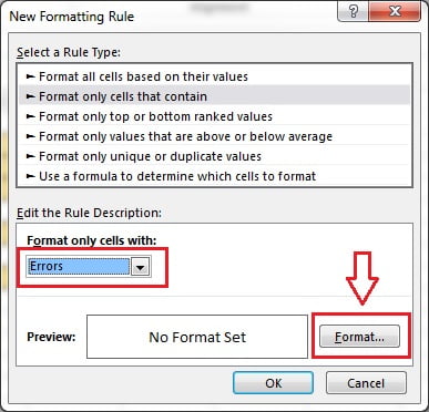
Errors formats cells that display any error value: #DIV/0!, #N/A, #NAME?, #VALUE!, #REF!, #NUM!, #NULL! and, in Excel 365, #SPILL!, #CALC! and #BLOCKED!. A common reporting trick is to set the font colour to match the background so errors vanish from print while the formula stays visible in the formula bar. Fixing the formula with IFERROR is usually better, but this rule tells you where the problems are in the first place.

No Errors formats every cell that does not hold an error. Use it when you want the good results shaded and the problem cells left plain for review, or to prove that a model has been cleaned up.

Worked example: a small order tracker

Four rules on one small table show how the options work together. Sample data in A1:D4, with today taken as 5 September 2026:

Order	Status	Due date	Value
ORD-101	Pending review	05/09/2026	148
ORD-102	Shipped	12/09/2026	192
ORD-103		04/09/2026	#DIV/0!

1. Select D2:D4, open New Rule > Format only cells that contain, set Cell Value greater than or equal to 150 and choose a green fill. ORD-102 turns green; ORD-101 does not, because 148 is below the limit.
2. Select B2:B4, add a rule with Specific Text containing Pending and an amber fill. ORD-101 is highlighted even though the cell reads Pending review, because containing matches anywhere in the text.
3. Select B2:B4 again and add a Blanks rule with a red border. The empty status cell on ORD-103 is boxed.
4. Select C2:C4 and add a Dates Occurring rule set to Today. ORD-101 is flagged. Select D2:D4 and add an Errors rule with a grey fill so ORD-103 shows as a data problem, not a real number.

The result is a tracker that keeps working as the data changes: a new order under 150 stays plain, a status typed into the blank cell removes the red border, and the Today highlight moves on by itself tomorrow.

When you need a formula rule instead

This rule type tests one condition against one cell. The moment you need two conditions, a comparison with another column, or a whole row highlighted, switch to Use a formula to determine which cells to format.

Write the formula for the top-left cell of the Applies to range; Excel copies it across the range like a fill, so the reference style decides what is tested. For example, select A2:D4 and enter =$B2="Shipped" to shade the whole row of every shipped order. Locking the column with $B2 means each cell in a row is tested against column B of its own row. B$2 locks the row instead and gives a whole-column highlight, and $B$2 locks both, which is what you want when the test points at a single input cell such as a search box, a drop-down or a checkbox.

Excel treats the result as TRUE or FALSE, and any non-zero number counts as TRUE. Two formulas worth remembering here: =AND(ISNUMBER(B2),B2>100) excludes text from a numeric test, and =AND($C2<>"",$C2<TODAY()) marks overdue dates while ignoring blank rows. One editing quirk catches everyone: inside the rule’s formula box the arrow keys insert cell references instead of moving the cursor. Press F2 first to switch to edit mode, then the arrow keys behave normally.

Errors and how to fix them

Problem	Cause	Fix
Greater than 100 also highlights text cells	Excel ranks any text above any number	Exclude the header, or use a formula rule with =AND(ISNUMBER(B2),B2>100)
Dates Occurring highlights nothing	The dates are text, not real dates	Check the alignment, then use Data > Text to Columns with Date in the last step, or DATEVALUE
Cell Value rules skip some numbers	Numbers stored as text, shown by a green corner triangle	Convert with Text to Columns or multiply by 1 in a helper column
Blanks highlights cells that look filled	The cell holds only spaces or a formula returning an empty string	Clean with TRIM, or use a formula rule such as =ISBLANK(B2) for true blanks only
The rule stopped working after rows were inserted	The Applies to range no longer covers the new rows	Open Manage Rules and widen Applies to, or convert the range to an Excel Table
Two rules fight over the same cell	The higher rule in the manager wins for the same property	Reorder with Move Up and Move Down, or use Stop If True

Tips and common mistakes

• Point the limits at input cells. =$J$1 and =$J$2 in the value boxes let anyone change the thresholds without opening the rule.
• Match the option to the data type. Cell Value reads the stored value and Specific Text reads the displayed characters, so a currency symbol never affects a numeric test.
• Equal to needs the whole cell. Pending review does not equal Pending. Use Specific Text containing for partial matches.
• Do not apply the same rule twice. Every OK adds another rule. Check Manage Rules and edit the existing one instead of stacking near-duplicates.
• Conditional formats cannot change font name or size, only style, colour, underline, strikethrough, border, fill and number format.
• Clear rules, do not paint over them. Filling a cell by hand leaves the rule alive underneath and it will reappear.
• Keep Applies to tight. Whole-column ranges such as B:B multiply the work Excel does on every recalculation and slow large files down.

Practice exercise

Open the course practice file or use any table of your own, then:

1. Apply Cell Value between 100 and 200 with a green fill, then edit the rule to not between and compare the result.
2. Change the two limits to references to cells J1 and J2, type new numbers there and confirm the highlights move.
3. Add a text column and apply Specific Text beginning with a two-letter code, then switch the rule to ending with.
4. Delete a few entries and apply Blanks with a red border, then No Blanks with a light fill on the same range.
5. Create a deliberate =1/0 somewhere in the range and add an Errors rule that hides it by setting the font colour to white.

Key takeaways

• Format only cells that contain tests each cell against itself using one of seven options.
• Cell Value gives all eight comparison operators, including greater than or equal to and not between.
• Specific Text offers containing, not containing, beginning with and ending with, and ignores case.
• Dates Occurring needs real dates and offers ten relative periods that roll forward automatically.
• Blanks, No Blanks, Errors and No Errors need no criteria at all, only a format.
• Value boxes accept cell references, so a rule can be driven by input cells such as =$J$1.
• For two conditions, a comparison with another column or a whole-row highlight, use a formula rule instead.

Related lessons

• Conditional Formatting course hub
• Highlight Cells Rules: the seven presets this dialog sits behind
• Use a formula to determine which cells to format
• Manage and clear conditional formatting rules
• Highlight dates: due today, overdue, this week and weekends
• Conditional formatting in pivot tables and highlighting errors, blanks and text
• IFERROR function for fixing the errors this rule finds
• COUNTIF function for counting the cells a rule would highlight
• Microsoft Support: Use conditional formatting to highlight information

Frequently asked questions

How is Format only cells that contain different from Highlight Cells Rules?

Highlight Cells Rules are one-click presets with six ready formats. This rule type is the dialog behind them, and it adds the greater than or equal to and less than or equal to operators, the not between test, the Blanks, No Blanks, Errors and No Errors options, and the full Format Cells dialog for number format, font, border and fill.

Can I combine two conditions in one rule?

Not with this rule type. It tests a single condition against a single cell. Use between or not between for a numeric range, or switch to Use a formula to determine which cells to format and join the tests with AND or OR, for example =AND(ISNUMBER($D2),$D2>150).

Why does greater than 100 highlight my text cells?

Excel sorts any text above any number, so a header or a comment passes a greater than test. Select only the numeric cells, or use a formula rule such as =AND(ISNUMBER(B2),B2>100) so the rule checks the data type first and the value second.

Does Specific Text accept wildcards such as an asterisk?

No. The containing test already matches the fragment anywhere in the cell, so an asterisk would be treated as a literal character. For pattern matching, use a formula rule built on SEARCH or COUNTIF, for example =COUNTIF($B2,"ORD-*")>0, which does support wildcards.

Why does the Blanks rule highlight a cell that looks filled?

The Blanks test trims the content first, so a cell holding only spaces counts as blank, and a formula returning an empty string does too. Clean the data with TRIM, or use a formula rule with =ISBLANK(B2) if you want only genuinely empty cells to be highlighted.

Want the finished version? Ready-made Excel KPI dashboards with target, variance and exception highlighting built in are available at NextGenTemplates.com.