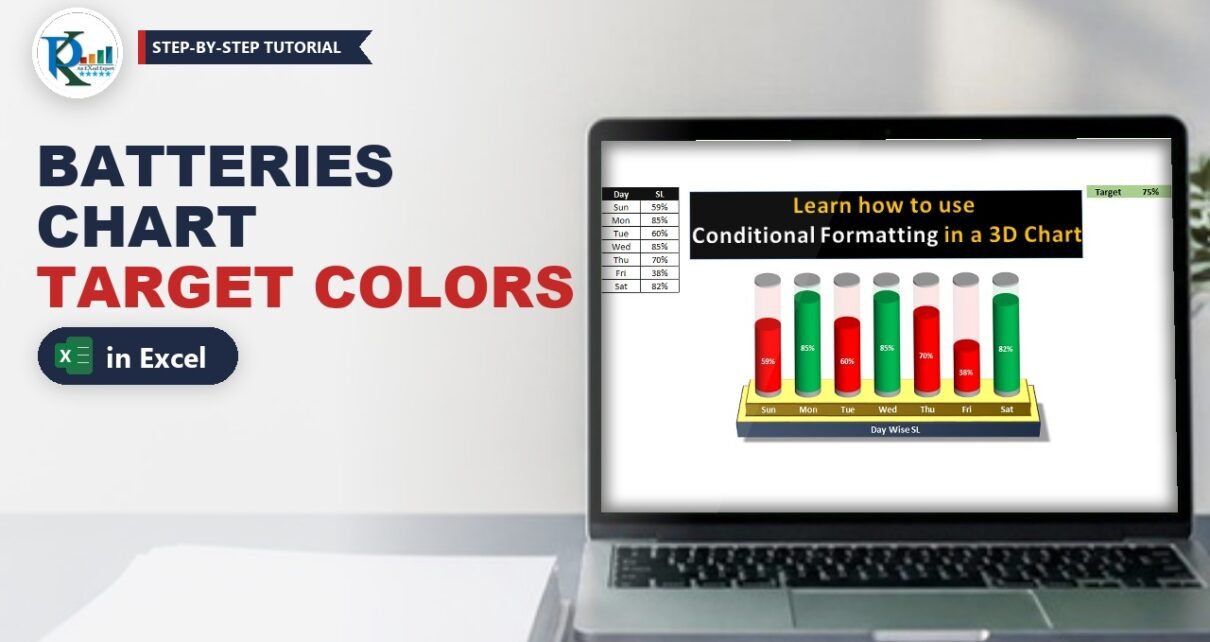
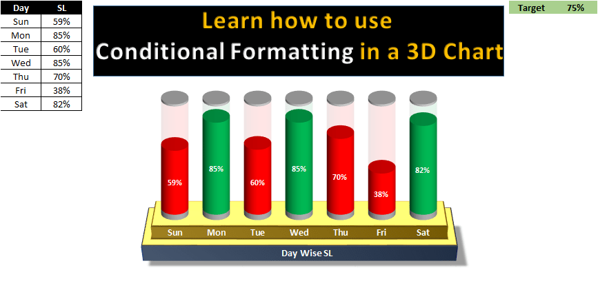
Conditional Formatting in Multiple Batteries Chart in Excel

Conditional formatting in a multiple batteries chart lets one Excel chart show several KPI values as 3D battery cells that turn green when the target is met and red when it is missed. In this tutorial you build a day-wise service level (SL) chart with seven batteries, a target cell, a few IF formulas and a 3-D stacked cylinder chart. Change any value or the target and every battery recolours itself instantly. There are no macros: the colour logic lives entirely in the data, which makes the chart fully dynamic and easy to reuse in dashboards.

Watch the Video Tutorial

In the video, PK sets up the helper columns, builds the 3-D stacked cylinder chart, colours the solid and transparent parts and finishes with a golden 3-D stand and a title.

What You Will Build

• A target-driven data table with one target cell that controls every colour.
• Green and Red helper columns that use IF and NA() to split each value into the right series.
• Transparent fill columns that complete every battery up to 100%.
• Grey caps at the top and bottom that make each cylinder look like a battery.
• A golden metal stand and a title for a polished, dashboard-ready finish.

Part 1 – Prepare the Data and Helper Columns

Step 1: Enter the values and the target

Put the days and service level in A1:B8 and the target next to the data. In the video the target label is in M1 and the value in N1:

Day   SL         M1: Target   N1: 70%
Sun   59%
Mon   68%
Tue   60%
Wed   51%
Thu   70%
Fri   38%
Sat   82%

Then type these headers in C1:H1: Bottom cap, Green, Red, Transparent Green, Transparent Red and Upper Cap. The order matters, because it becomes the stacking order of the chart from bottom to top.

Step 2: The caps

Enter 3% in every row of column C (Bottom cap) and column H (Upper Cap). These thin slices become the grey metal ends of each battery.

Step 3: Split the value into Green or Red

In D2 and E2 enter:

D2  =IF(B2>=$N$1,B2,NA())
E2  =IF(B2<$N$1,B2,NA())

Press F4 on N1 so the target reference stays fixed, fill both formulas down to row 8 and format them as percentages.

Step 4: The transparent part

The empty part of each battery is whatever is left up to 100%:

F2  =1-D2
G2  =1-E2

Fill them down. Some cells show #N/A, and that is expected. Ignore those errors; the chart needs them.

How the formula works

• B2>=$N$1 checks if the day met the target. If it did, the value goes into the Green column; otherwise Green gets NA().
• The Red formula uses the opposite test, so every value lands in exactly one of the two columns.
• A chart does not draw #N/A, so each battery shows only one coloured segment.
• 1-D2 and 1-E2 fill the battery up to 100%. If D2 is #N/A, F2 is #N/A too, so only the matching transparent colour appears above the coloured part.
• Because the colour comes from the data, changing the target in N1 recolours the whole chart. That is how you get conditional formatting in a chart without VBA.

Part 2 – Build the Multiple Batteries Chart

Step 5: Insert a 3-D stacked column chart

Select A1:A8, hold Ctrl and select C1:H8 (the Bottom cap to Upper Cap columns, without SL). Go to Insert > Column Chart > 3-D Stacked Column. With the Chart Elements (+) button remove the chart title, gridlines and legend, then click the vertical axis and press Delete.

Step 6: Turn the columns into cylinders

Right-click a column > Format Data Series > Series Options. Choose the Cylinder column shape, reduce the Gap Width so the batteries look a little wider, and set Gap Depth to 0.

Part 3 – Conditional Formatting in the Multiple Batteries Chart

Step 7: Colour each series

Select each series in turn (click it in the chart) and set its fill in Format Data Series > Fill:

• Bottom cap and Upper Cap: light grey (White, Background 1, Darker 25%).
• Red: solid red.
• Transparent Red: the same red with 75% transparency.
• Green: solid green.
• Transparent Green: the same green with 75% transparency.

Tip from the video: the transparent parts are hard to see on white, so temporarily fill the chart area black while you pick them, then set it back.

Step 8: Add data labels

Right-click the red series > Add Data Labels, then set the labels to font size 11, white and bold. Do the same for the green series. Only the visible segment shows a label, because #N/A points have no label.

Step 9: Tilt the chart

Right-click the chart area > 3-D Rotation and set X Rotation 0° and Y Rotation 20° (PK tries 30° first, then settles on 20°) so you look slightly down onto the caps. Make the horizontal axis labels size 11 and bold.

Test it: change the target in N1 to 50% and every day above 50% turns green at once.

Step 10: Clean background

Select the chart and set Fill > No fill and Border > No line. On the View tab untick Gridlines and Headings.

Part 4 – Add the 3-D Stand and Title

Step 11: Draw the golden stand

1. Insert a Rectangle under the chart, fill it gold and give it a dark blue outline.
2. In Format Shape > Effects > 3-D Rotation, choose the preset Perspective Relaxed.
3. In 3-D Format, set the Top bevel to Cross with Width 25 pt and Height 25 pt, Depth 20 pt, Material Metal and Lighting angle 20°.
4. Right-click the shape > Send to Back and position the chart on top of it. Change the axis labels to white so they read clearly on the gold.

Step 12: Add a title

Insert a Text Box on the front edge of the stand, type Day wise SL, make it bold with a white font, and set Shape Fill and Shape Outline to none.

Common Errors and Fixes

These fixes are additions based on general Excel behaviour, not shown in the video.

A value equal to the target shows red

Check the Green formula uses >= and the Red formula uses <. With those operators, a value exactly on target is green, as Thursday at 70% is in the video.

Both colours appear in one battery

One helper formula returns 0 or blank instead of NA(). Use NA() as the false result, because a zero still creates a stacked segment and label.

The batteries are taller than 100%

That is normal: the two 3% caps add 6% on top of 100%. Keep both caps the same size for every row so all batteries end at the same height.

I cannot find the Cylinder option

The column shape appears in Format Data Series only for 3-D column charts. Make sure you inserted the 3-D Stacked Column, not the 2-D stacked column.

Tips

• Put the target in a clearly labelled cell so managers can change it without touching formulas.
• Add a third band (for example amber within 5% of target) with one more pair of solid and transparent columns.
• Use the same layout for weekly, monthly or agent-wise KPIs; just extend the rows.
• Group the chart, stand and title so they move together on a dashboard.
• Microsoft explains the NA function and the IF function used in the helper columns.

Want It Ready-Made?

If you want the finished workbook with the batteries, colours and stand already built, get the Conditional Formatting in Multiple Batteries Chart template, or browse more Excel chart templates on NextGenTemplates.com. To build dynamic charts and KPI dashboards step by step, join the course Excel Pivot Tables and Dashboards on NextGenTemplates Academy.

Related Tutorials

• Battery Chart in Excel
• Stunning Battery Chart in Excel
• 5 KPI Cylinder Chart in Excel
• RAG Conditional Formatting in a 3D Chart
• Conditional Formatting in an Excel Chart

Frequently Asked Questions

Can you apply conditional formatting to a chart in Excel?

Not directly, but you can get the same effect by splitting the data into separate series with IF formulas. Each series has its own colour, so the colour follows the rule automatically.

Why use NA() instead of 0 or blank?

A chart ignores #N/A values, so no segment or label is drawn. A zero would still create a stacked point and an unwanted label.

How do I change the target for all batteries?

Type a new value in the target cell. All the Green and Red formulas refer to it with an absolute reference, so every battery recolours at once.

What makes the columns look like batteries?

The 3-D stacked column with the Cylinder shape, thin grey caps at the top and bottom, and a 75% transparent segment that shows the empty part of each cell.

Does this chart need VBA?

No. It is driven only by formulas and chart formatting, so it works in a normal xlsx workbook.

About the Author

PK is a Microsoft Excel expert and trainer and the founder of PK: An Excel Expert and NextGenTemplates.com. He has been teaching Excel, Power Query and Power BI since 2016 on his YouTube channel.

Conclusion

Conditional formatting in a multiple batteries chart comes down to one idea: let IF and NA() decide which series each value belongs to, then give those series their own colours. Add transparent fill columns, grey caps, a cylinder shape and a 3-D stand, and you have a target-aware KPI visual that updates itself whenever the data or the target changes.