Highlight Duplicate or Unique Values in Excel: Rules and Formulas

Part of the free Module 7: Conditional Formatting · Lesson 10 of 15 · Full Excel course

Updated on 5 September 2026 · Works in Excel 365, 2021, 2019 and 2016 unless noted.

Format only unique or duplicate values is the conditional formatting rule in Excel that highlights every value appearing more than once in the selected range, or, switched to unique, every value that appears exactly once. You reach it through Home > Conditional Formatting > New Rule, and it gives you the full Format Cells dialog instead of the six preset colours.

What the rule does

Excel compares each cell in the Applies to range with every other cell in that same range. A cell counts as a duplicate when at least one other cell holds the same value, and as unique when no other cell matches. Both copies of a repeated value are highlighted, not just the second one, so a value that appears three times lights up three cells.

Use the duplicate option to catch repeated invoice numbers, employee IDs, email addresses or part codes before they reach a report. Use the unique option to spot one-off entries, such as a customer who ordered only once or a code that was typed by hand. The rule is live: paste a repeated ID and the highlight appears on the next recalculation, with no need to reopen the dialog.

How the rule counts across the Applies to range

This is the part that surprises people. The comparison is made across the whole Applies to range, not column by column and not row by row. If you select B2:G9, a value in D5 is compared with all 48 cells, so a number that appears once in Location-1 and once in Location-3 is a duplicate. That is exactly what you want for a grid of readings, and exactly what you do not want when you meant to check one column only.

If you need a per-column check, apply a separate rule to each column, or type the column addresses into the Applies to box separated by commas: =$B$2:$B$9,$D$2:$D$9. Each contiguous block is still compared as one pool, so keep the ranges you want compared together in the same rule and split the ones you do not.

Question	How the rule behaves
Is the first occurrence highlighted?	Yes. Every copy is formatted, including the first.
Is text matching case-sensitive?	No. abc, Abc and ABC are all the same value.
Are 100 and the text 100 duplicates?	No. A number and a number stored as text are different values.
Do trailing spaces matter?	Yes. ABC and ABC followed by a space are different values.
Are blank cells treated as duplicates?	No. Empty cells are ignored by the rule.
Does the comparison respect the number format?	No. 1.0 and 1.00 are the same underlying number and count as duplicates.
Are whole rows compared?	No. Only single cell values are compared, never a combination of columns.

Step by step: highlight duplicate values

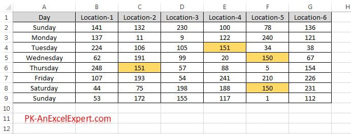
The example uses a day-wise, location-wise sales table in B2:G9.

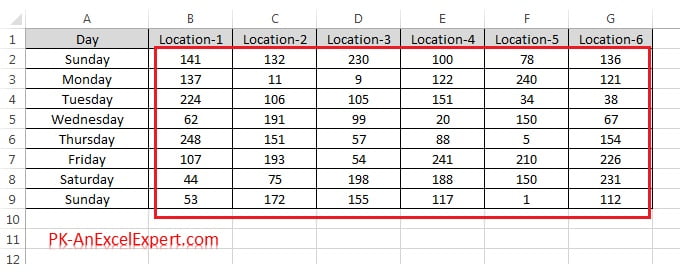
1. Select the range B2:G9. Leave out the header row and the day labels so text is not thrown into the same comparison pool as the numbers.
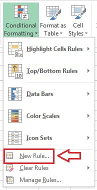
2. Go to Home > Conditional Formatting > New Rule.

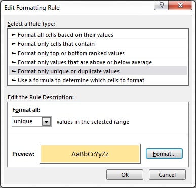
3. In the New Formatting Rule dialog select Format only unique or duplicate values, then choose duplicate in the Format all drop-down.

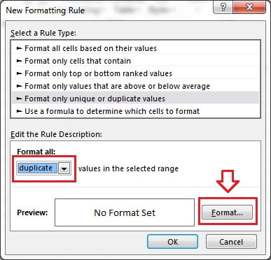
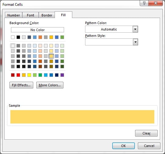
4. Click Format, pick a fill colour on the Fill tab of the Format Cells dialog and click OK. You can also set a font colour, a bold style, a border or a number format here.

5. Click OK again. Every value that occurs more than once anywhere in B2:G9 is highlighted.

Highlight unique values instead

1. Select the same range and open New Rule again, or open Manage Rules and click Edit Rule on the rule you already made.
2. Keep the rule type and switch the Format all drop-down to unique.

3. Click Format, choose a different fill so the two rules are easy to tell apart, then click OK twice.

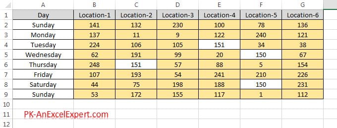
Duplicate and unique are opposites over the same range, so applying both with different colours leaves no cell unformatted except blanks. That is a quick way to prove to yourself that the rule really is scanning the whole selection.

This rule or the Duplicate Values preset?

Home > Conditional Formatting > Highlight Cells Rules > Duplicate Values produces exactly the same result in one click, and it is the right choice when you are in a hurry. The comparison logic is identical in both places, because the preset simply creates this rule type for you. The difference is the format.

Point of difference	Duplicate Values preset	Format only unique or duplicate values
Where it lives	Highlight Cells Rules menu	New Rule dialog
Formats offered	Six ready-made fill and font combinations	Full Format Cells dialog: number, font, border, fill
Clicks to apply	Two	Four
Underlying rule type	Format only unique or duplicate values	Format only unique or duplicate values
Best for	A quick check you will clear again	A report format you will keep, in brand colours

Because the preset creates the same rule, you can start with the preset and then open Manage Rules > Edit Rule to reach the full Format Cells dialog without rebuilding anything.

Formula equivalents that go further

The built-in rule cannot flag only the second occurrence, and it cannot compare two columns together. A formula rule can do both. Choose New Rule > Use a formula to determine which cells to format and enter one of these.

Goal	Formula
All duplicates in column B, same as the built-in rule	=COUNTIF($B$2:$B$21,$B2)>1
Second and later occurrences only, leaving the first copy clean	=COUNTIF($B$2:$B2,$B2)>1
Duplicate rows judged on two columns together	=COUNTIFS($B$2:$B$21,$B2,$C$2:$C$21,$C2)>1
Values that appear only once in column B	=COUNTIF($B$2:$B$21,$B2)=1
Values that also appear on another sheet	=COUNTIF(Sheet2!$A:$A,$B2)>0

The reference pattern is the whole trick. Excel writes the formula for the top-left cell of the Applies to range and then copies it across that range like a fill, so relative parts shift and locked parts do not. $B$2:$B$21 is locked at both ends and stays the pool that every cell is counted against. $B2 locks the column but lets the row move, so every cell in row 5 is tested against B5. That single dollar sign is what turns a one-column highlight into a whole-row highlight: set Applies to as =$B$2:$F$21 and use =COUNTIF($B$2:$B$21,$B2)>1, and the entire record is coloured when its ID repeats. Lock the row instead, as B$2, to colour a whole column, and lock both, as $B$2, when the formula must always point at one input cell.

Excel treats the result as TRUE or FALSE, and any non-zero number counts as TRUE. One practical detail in the rule dialog: press F2 before you use the arrow keys inside the formula box, otherwise the arrows insert cell references instead of moving the cursor.

=COUNTIF($B$2:$B2,$B2)>1 deserves a second look. The first end of the range is locked and the second is relative, so the range grows as the rule is copied down: in row 2 it counts B2:B2, in row 7 it counts B2:B7. The count can only exceed 1 once a value has already been seen above, which is why the first copy stays clean and every repeat is highlighted. That is the version you want when you are about to delete duplicates by hand.

Worked example: duplicate order IDs

An order log has an ID in column B and a customer in column C.

Row	B: Order ID	C: Customer	All duplicates	Repeats only
2	SO-1001	Acme	Highlighted	Clean
3	SO-1002	Brightway	Highlighted	Clean
4	so-1001	Acme	Highlighted	Highlighted
5	SO-1003	Acme	Clean	Clean
6	SO-1002	Cortex	Highlighted	Highlighted

1. Select B2:B6 and apply Format only unique or duplicate values with duplicate. Rows 2, 3, 4 and 6 are highlighted: the check ignores case, so so-1001 matches SO-1001, and SO-1002 appears twice. Only SO-1003 in row 5 is left clean, and switching the rule to unique would colour that one cell alone.
2. Now select B2:C6, add a formula rule =COUNTIFS($B$2:$B$6,$B2,$C$2:$C$6,$C2)>1 and give it a border. Only rows 2 and 4 are bordered, because they are the only pair that matches on ID and customer together. The two SO-1002 rows belong to different customers, so they are separate orders rather than a double entry.
3. Add a third rule on B2:B6 with =COUNTIF($B$2:$B2,$B2)>1 in red. Rows 4 and 6 turn red: the second copy of each ID, the ones you would delete, while the first copy of each stays clean.

From highlighting to cleaning: Remove Duplicates and UNIQUE

Conditional formatting only colours cells. It never changes or deletes data, so treat it as the review step and follow it with one of these.

1. Review first. Apply the duplicate rule and read the highlighted rows. Genuine repeats and legitimate repeats look identical to Excel, so a human check matters.
2. Delete in place with Remove Duplicates. Select the range, go to Data > Data Tools > Remove Duplicates, tick only the columns that define a duplicate for you, and click OK. Ticking Order ID and Customer matches the COUNTIFS rule above. Excel keeps the first occurrence and reports how many rows it removed. This edits the data, so work on a copy.
3. Keep the original and spill a clean list. In Excel 365 and 2021, =UNIQUE(B2:B21) returns each value once into a spilled range, and =UNIQUE(B2:C21) returns distinct row combinations. Add the third argument, =UNIQUE(B2:B21,,TRUE), to return only the values that appear exactly once, which is the list version of the unique highlight.
4. Count before you cut. =SUMPRODUCT((COUNTIF(B2:B21,B2:B21)>1)*1) tells you how many cells the duplicate rule has highlighted, and =COUNTA(B2:B21)-COUNTA(UNIQUE(B2:B21)) tells you how many rows Remove Duplicates would delete.

Tips and common mistakes

• Trailing spaces break the match. A value typed with a space at the end is a different value. Clean the column with TRIM or Find and Replace before you trust the highlights.
• Numbers stored as text never match real numbers. The green triangle in the corner is the warning. Fix them with Data > Text to Columns or the VALUE function.
• Do not include headers in the selection. A repeated header word joins the comparison pool and is highlighted as a duplicate.
• Filtering does not shrink the comparison pool. Hidden and filtered rows stay inside the Applies to range, so a row you cannot see can still be the reason a visible cell is highlighted.
• Check the Applies to range after copy and paste. Pasting cells inside the range often splits one rule into several fragments. Open Manage Rules and consolidate them.
• Highlighting is not deleting. Remove Duplicates is a separate command under the Data tab and it changes the data permanently.
• Text longer than 255 characters is compared on the first 255 only, so long descriptions can appear as duplicates when only their openings match.

Errors and how to fix them

Symptom	Likely cause	Fix
Two identical looking cells are not both highlighted	A trailing space, or one value is text and the other a number	Test with =EXACT(B2,B5) and =LEN(B2), then TRIM or convert
Far more cells highlight than expected	The Applies to range covers several columns and values repeat across them	Narrow Applies to, or create one rule per column
The first occurrence is coloured too	Normal behaviour of the built-in rule	Use the formula rule =COUNTIF($B$2:$B2,$B2)>1
Nothing highlights on an obvious repeat	Case differences are not the cause; a non-breaking space or an apostrophe prefix usually is	Retype one cell and compare, or use =CLEAN(TRIM(B2)) in a helper column
The rule disappears after inserting a row	The insert split the Applies to range	Reset Applies to in Manage Rules, or convert the data to an Excel Table
Formula rule returns an error and refuses to save	The formula is missing the leading equals sign, or refers to another workbook	Start with =; conditional formatting cannot reference another workbook

Practice exercise

Open the course practice file or use any list of IDs, then:

1. Apply Format only unique or duplicate values to B2:G9 with a yellow fill for duplicates, and count how many cells highlight.
2. Edit the rule to unique with a green fill and confirm that the two rules together cover every non-blank cell.
3. Change the Applies to range to a single column and note how many fewer cells now qualify as duplicates.
4. Add a formula rule =COUNTIF($B$2:$B2,$B2)>1 in red and check that only the repeats are red.
5. Type a value as text with a leading apostrophe, confirm it does not match the numeric copy, then convert it and watch the highlight appear.
6. Finish with Data > Remove Duplicates on a copy of the sheet and compare the row count with =UNIQUE(B2:B21).

Key takeaways

• Format only unique or duplicate values compares every cell in the Applies to range with every other cell in that range, across all its columns.
• Every copy of a repeated value is highlighted, including the first, and text matching ignores case.
• Numbers stored as text, trailing spaces and blanks are the three usual reasons a match fails.
• The Duplicate Values preset creates the same rule but limits you to six formats; New Rule gives the full Format Cells dialog.
• =COUNTIF($B$2:$B2,$B2)>1 flags repeats only, and =COUNTIFS(...) flags duplicate rows on several columns.
• Lock the column as $B2 to highlight the whole row from one key column.
• Highlighting reviews the data; Remove Duplicates and UNIQUE are what actually clean it.

Related lessons

• Conditional Formatting course hub
• Highlight Cells Rules, including the Duplicate Values preset
• Use a formula to determine which cells to format
• Manage and clear conditional formatting rules
• COUNTIF function and COUNTIFS function
• Stop duplicates being typed at all with a custom data validation rule
• Microsoft Support: Highlight patterns and trends with conditional formatting

Frequently asked questions

Why does the rule highlight the first occurrence as well?

Because the built-in rule asks a question about the value, not about position: does this value appear more than once in the range. Both copies answer yes, so both are formatted. To leave the first copy clean, use a formula rule with an expanding range, =COUNTIF($B$2:$B2,$B2)>1, which can only be true once the value has already been seen above.

How do I highlight duplicate rows rather than duplicate cells?

The built-in rule never compares combinations of columns. Use a formula rule instead. Set Applies to across the whole record, for example =$B$2:$F$21, and enter =COUNTIFS($B$2:$B$21,$B2,$C$2:$C$21,$C2)>1. Add another pair of arguments for each extra column that has to match. The dollar signs on the column letters keep every cell in a row testing the same two key columns.

Is the duplicate check case-sensitive?

No. Excel treats abc, Abc and ABC as the same value, so all three are marked as duplicates. If case matters, use a formula rule built on EXACT and SUMPRODUCT, for example =SUMPRODUCT(--EXACT($B$2:$B$21,$B2))>1, which compares character by character and respects capitals.

How do I find duplicates between two sheets?

The rule only looks inside its own Applies to range, so switch to a formula rule. Select the range on the first sheet and enter =COUNTIF(Sheet2!$A:$A,$B2)>0. Conditional formatting can reference another sheet in the same workbook from Excel 2010 onwards, but it cannot reference a different workbook; copy the other list into the same file first.

Does highlighting duplicates delete them?

No. Conditional formatting only changes appearance. To remove repeats, select the range and use Data > Data Tools > Remove Duplicates, ticking the columns that define a duplicate, which keeps the first occurrence. In Excel 365 and 2021 you can instead spill a clean list beside the data with =UNIQUE(B2:B21) and leave the original untouched.

Want the finished version? Ready-made Excel KPI dashboards and trackers with duplicate checks and validation built in are available at NextGenTemplates.com.