Above or Below Average Conditional Formatting in Excel

Part of the free Module 7: Conditional Formatting · Lesson 9 of 15 · Full Excel course

Updated on 5 September 2026 · Works in Excel 365, 2021, 2019 and 2016 unless noted.

Format only values that are above or below average is the conditional formatting rule type that compares every cell with the average of the range the rule is applied to, then formats the cells above it, below it, or one, two or three standard deviations away from it. Because the average is recalculated from the data itself, the highlight moves as the numbers change.

What the above or below average rule does

Excel works out the mean of every numeric cell in the Applies to range, compares each cell with that mean, and formats the cells that pass the test you picked. Nothing is typed as a threshold, so the benchmark is the data. That is the point of the rule: a fixed target such as 150 has to be edited every time the business changes, while an average-based rule keeps working on its own.

Use it when the question is comparative rather than absolute. Which stores beat the regional average? Which handling times sit below the team mean? Which readings are far enough from the middle to count as outliers? The rule behaves the same way in Excel 2016 through Microsoft 365, and the dialog has not changed.

The ten comparison options

The drop-down in the New Formatting Rule dialog holds ten options. The third column shows the formula rule that produces the same result on a list in B2:B21, which is useful when you need the logic somewhere the built-in rule cannot reach.

Option	Formats cells that are	Equivalent formula rule
above	Greater than the average, average itself excluded	=B2>AVERAGE($B$2:$B$21)
below	Less than the average, average itself excluded	=B2<AVERAGE($B$2:$B$21)
equal or above	Greater than or equal to the average	=B2>=AVERAGE($B$2:$B$21)
equal or below	Less than or equal to the average	=B2<=AVERAGE($B$2:$B$21)
1 std dev above	Above the mean plus one standard deviation	=B2>AVERAGE($B$2:$B$21)+STDEV.P($B$2:$B$21)
1 std dev below	Below the mean minus one standard deviation	=B2<AVERAGE($B$2:$B$21)-STDEV.P($B$2:$B$21)
2 std dev above	Above the mean plus two standard deviations	=B2>AVERAGE($B$2:$B$21)+2*STDEV.P($B$2:$B$21)
2 std dev below	Below the mean minus two standard deviations	=B2<AVERAGE($B$2:$B$21)-2*STDEV.P($B$2:$B$21)
3 std dev above	Above the mean plus three standard deviations	=B2>AVERAGE($B$2:$B$21)+3*STDEV.P($B$2:$B$21)
3 std dev below	Below the mean minus three standard deviations	=B2<AVERAGE($B$2:$B$21)-3*STDEV.P($B$2:$B$21)

Microsoft does not document which standard deviation variant the built-in rule uses. In testing it matches the population form, STDEV.P, taken over the whole Applies to range. If you need to be certain which measure is behind a report, build the rule as a formula rule so the choice between STDEV.P and STDEV.S is yours and visible.

What the average is calculated over

The average comes from the rule’s Applies to range, not from the column, the sheet or the visible rows. Four consequences are worth remembering:

• Blank cells and text are ignored. They are not counted as zero and they do not change the mean, exactly as the AVERAGE function behaves. Logical TRUE and FALSE values in cells are ignored too.
• Zeros do count. A column padded with placeholder zeros drags the average down and pushes ordinary values above it.
• Filtered and hidden rows still count. Conditional formatting evaluates the whole range, so filtering the list does not recalculate the average against what you can see.
• Select one block, get one average. If the Applies to range covers six columns, all six share a single mean. Per-column averages need one rule per column or the formula rule shown later.

The mean is live. Edit any value in the range and Excel recalculates it, so highlights can appear on cells you did not touch. New rows only join the calculation if they fall inside the Applies to range, which is the main argument for putting the data in an Excel Table before you add the rule.

Step by step: highlight above-average values

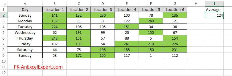
The example uses a day-wise, location-wise sales table in B2:G9.

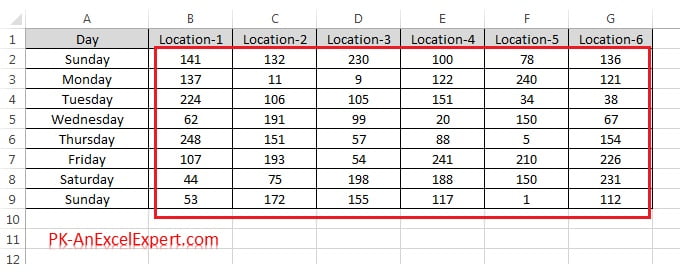
1. Select the numeric range B2:G9. Leave out the header row and the day labels, or the text will simply be ignored and the selection will be harder to edit later.
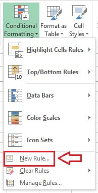
2. Go to Home > Styles > Conditional Formatting > New Rule.

3. In the New Formatting Rule dialog, choose the rule type Format only values that are above or below average, then set the drop-down under Format values that are to above the average for the selected range.

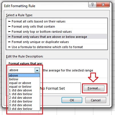
4. Click Format, pick a fill colour on the Fill tab of the Format Cells dialog and click OK. You can set the number format, font style, colour, underline and border here, but not the font name or size.

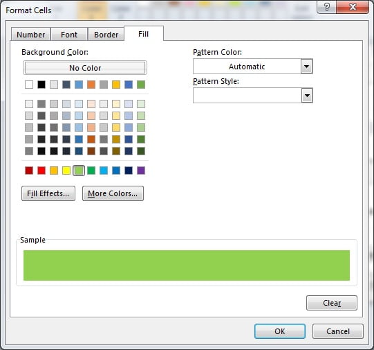
5. Click OK again. Every value greater than the average of B2:G9 is formatted, and cells exactly equal to the average are not.

Highlight below-average values

Add a second rule to the same range so the two formats work together as a variance view.

1. Select B2:G9 again and open Conditional Formatting > New Rule.
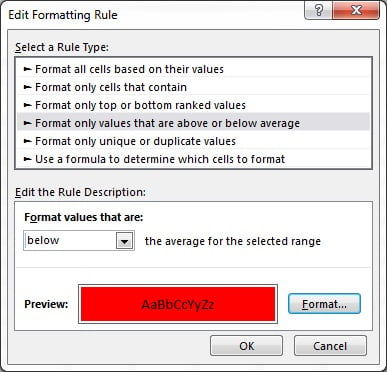
2. Choose the same rule type and set the drop-down to below.

3. Click Format, choose a contrasting fill such as light red, then click OK twice.

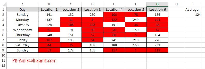
The two rules never fight, because no cell can be above and below the same mean at once. Cells sitting exactly on the average stay unformatted; switch one rule to equal or above if you want them included.

Using the standard deviation options

Standard deviation measures how spread out the numbers are. Roughly two thirds of a normally distributed data set sits within one standard deviation of the mean, about 95 per cent within two, and about 99.7 per cent within three. That gives the options a practical reading: 1 std dev above marks the strong performers, 2 std dev above marks the genuinely unusual, and 3 std dev either way is close to an alarm.

Business data is rarely a perfect bell curve, so treat the percentages as a guide rather than a promise. Skewed data such as invoice values or call durations often has a long tail, and a single very large value inflates both the mean and the standard deviation, which can leave the 2 std dev rule highlighting nothing at all. When that happens, top or bottom ranked rules are usually the better tool.

The equivalent formula rules and how the references work

Every option in this rule type can be rebuilt with Use a formula to determine which cells to format. That matters when you need a whole row highlighted, an average from a different range, or a sample rather than a population standard deviation. For a list of 20 order values in B2:B21, select B2:B21 and enter:

=B2>AVERAGE($B$2:$B$21)
=B2>AVERAGE($B$2:$B$21)+STDEV.P($B$2:$B$21)

Write the formula for the top-left cell of the Applies to range. Excel then copies it across the rest of the range exactly like a fill, adjusting the relative parts and leaving the locked parts alone. So B2 is relative, which is what makes each cell test its own value, while $B$2:$B$21 is locked so all 20 cells are measured against the same average. Leave the dollar signs off the average range and Excel shifts the window down as it copies, giving every row a different benchmark and a meaningless result.

The rule fires when the formula evaluates to TRUE. Any non-zero number also counts as TRUE, and 0 or FALSE counts as FALSE. The same locking logic drives the other layouts:

• =$B2>AVERAGE($B$2:$B$21) locks the column only, so every cell in a row is tested against column B of its own row. Apply it to A2:F21 to highlight the whole row of an above-average order.
• =B$2>AVERAGE($B$2:$G$2) locks the row only, which tests a whole column against a value in row 2.
• =$B$2>AVERAGE($B$5:$B$24) locks both, the form to use when the comparison depends on one input cell such as a search box, drop-down or checkbox.

One practical warning about the formula box: it starts in point mode, so pressing an arrow key inserts a cell reference instead of moving the cursor. Press F2 first to switch to edit mode, then the arrow keys move through the formula normally.

Give every column its own average

The built-in rule gives one average to the whole selection, which is wrong whenever the columns are not comparable, for example three locations with very different volumes. A single formula rule solves it. Select B2:G9, choose Use a formula to determine which cells to format, and enter:

=B2>AVERAGE(B$2:B$9)

The column letter is relative, so as Excel copies the formula sideways it becomes C2>AVERAGE(C$2:C$9), then D, and so on. The row numbers are locked with dollar signs, so every column keeps looking at rows 2 to 9. The result is six independent averages from one rule. Swap the axes with =B2>AVERAGE($B2:$G2) and each row is compared with its own average instead.

Worked example

Ten sales representatives with their monthly totals in B2:B11:

Representative	Sales	Above or below the mean of 470
Amit	420	Below
Bhavna	505	Above
Chetan	388	Below, and 1 std dev below
Deepa	610	Above, and 1 std dev above
Farid	455	Below
Gita	372	Below, and 1 std dev below
Harsh	528	Above
Isha	441	Below
Jai	396	Below
Kiran	585	Above, and 1 std dev above

1. Select B2:B11 and apply the rule with above and a green fill. Four cells turn green: 505, 610, 528 and 585, because the total is 4,700 and the average is 470.
2. Add a second rule with below and a light red fill. The other six cells turn red.
3. Add a third rule with 1 std dev above and a bold font. The population standard deviation of these ten values is about 79.2, so the threshold is 470 plus 79.2, or 549.2. Only 610 and 585 qualify.
4. Add a fourth rule with 1 std dev below. The threshold is 390.8, so 388 and 372 qualify.
5. Try 2 std dev above. The threshold is 628.4 and nothing is highlighted, which is the honest answer for a data set this tight.

Change Kiran to 950 and watch every result move: the average rises to 506.5, Bhavna drops out of the green set, and the standard deviation grows enough that 610 stops counting as an outlier. That sensitivity to one large value is the single most important thing to understand about average-based rules.

Tips and common mistakes

• Do not include totals in the range. A grand total inside the Applies to range distorts the mean badly and is always highlighted as above average.
• Strip placeholder zeros. Zeros are averaged, blanks are not, so a column of dashes typed as 0 pulls the benchmark down.
• Check for numbers stored as text. Left-aligned figures with a green triangle are ignored by the rule and by AVERAGE. Fix them with Data > Text to Columns before formatting.
• Use equal or above deliberately. With whole numbers a cell can land exactly on the average, and above alone leaves it unformatted.
• Convert the data to a Table. The Applies to range then grows with new rows automatically, so the average stays honest as the list expands.
• Do not run the rule twice. Each pass through the dialog creates a new rule. Check Home > Conditional Formatting > Manage Rules before adding another.
• Prefer a fixed threshold when there is a real target. If the business rule is 150 units, use Format only cells that contain, not an average that drifts every month.

Errors and how to fix them

What you see	Cause	Fix
Almost every cell is highlighted as above average	One very small value, or a block of zeros, is dragging the mean down	Remove the zeros or exclude the outlier row from the Applies to range
2 or 3 std dev rules highlight nothing	The spread is small, or one big value has inflated the standard deviation	Use 1 std dev, or switch to a top or bottom ranked rule
Filtering the list does not change the highlights	Conditional formatting evaluates hidden rows as well	Copy the filtered rows to a new sheet, or use a formula rule with SUBTOTAL
New rows are not formatted	The Applies to range still ends at the old last row	Edit Applies to in Manage Rules, or convert the range to an Excel Table
Columns with different scales all compare with one mean	A single rule covers the whole block	Use the per-column formula rule =B2>AVERAGE(B$2:B$9)
The formula box inserts references when you press an arrow key	The box is in point mode	Press F2 to switch to edit mode, then use the arrow keys

Practice exercise

Open the course practice file or use any table of numbers, then:

1. Apply above in green and below in light red to the whole sales block, then change one figure and confirm several highlights move at once.
2. Add a 2 std dev above rule with a bold border and note how few cells, if any, qualify.
3. Type =AVERAGE(B2:G9) and =STDEV.P(B2:G9) in spare cells and check that the highlights match the thresholds you calculate.
4. Replace the built-in rule with the formula rule =B2>AVERAGE(B$2:B$9) and compare which cells change colour.
5. Convert the range to a Table with Ctrl+T, add a row and confirm the new value joins the average automatically.

Key takeaways

• The rule compares every cell with the mean of the Applies to range and offers above, below, equal or above, equal or below and 1, 2 or 3 standard deviations either side.
• Blanks and text are ignored, zeros are counted, and hidden or filtered rows still take part in the average.
• One rule gives one average to the whole selection, so unequal columns need one rule each or a formula rule.
• Every option can be rebuilt as a formula rule, for example =B2>AVERAGE($B$2:$B$21) or =B2>AVERAGE($B$2:$B$21)+STDEV.P($B$2:$B$21).
• Dollar signs decide the shape of the highlight: lock the column for whole rows, the row for whole columns, and both for a single input cell.
• Average-based rules move with the data, which is their strength for benchmarking and their weakness when a target is fixed.

Related lessons

• Conditional Formatting course hub
• Top/Bottom Rules: the Above Average and Below Average presets
• Format only top or bottom ranked values
• Use a formula to determine which cells to format
• Rule precedence and Stop If True
• Excel formulas course for AVERAGE, STDEV.P and the statistical functions
• Microsoft Support: Highlight patterns and trends with conditional formatting

Frequently asked questions

What average does the rule actually use?

The arithmetic mean of every numeric cell inside the rule’s Applies to range. Blank cells and text are skipped, zeros are included, and hidden or filtered rows still count. If the rule covers six columns, all six share one mean. Check the figure by typing AVERAGE over the same range in a spare cell.

Does the average update when I add new data?

Yes, but only for cells inside the Applies to range. Rows added below the range are ignored until you extend it in Manage Rules. The reliable fix is to convert the data to an Excel Table with Ctrl+T before applying the rule, because the Applies to range then grows with the Table.

Which standard deviation does Excel use for these options?

Microsoft does not state it in the documentation. In testing the built-in rule matches the population standard deviation, STDEV.P, over the Applies to range. Where the distinction matters, build the rule as a formula rule so you can choose STDEV.P or STDEV.S yourself and show the working on the sheet.

How do I compare each column with its own average?

Use a formula rule instead of the preset. Select the block, choose Use a formula to determine which cells to format and enter the formula with the column letter relative and the row numbers locked, such as the one that averages B$2:B$9. Excel then shifts the reference sideways and every column gets its own benchmark.

Why is a cell equal to the average left unformatted?

The above and below options are strict comparisons, so a value sitting exactly on the mean fails both tests. Choose equal or above, or equal or below, when the boundary value should be included. This happens most often with small sets of whole numbers where the average lands on a round figure.

Want the finished version? Ready-made Excel KPI dashboards with average, variance and outlier highlighting already built in are available at NextGenTemplates.com.