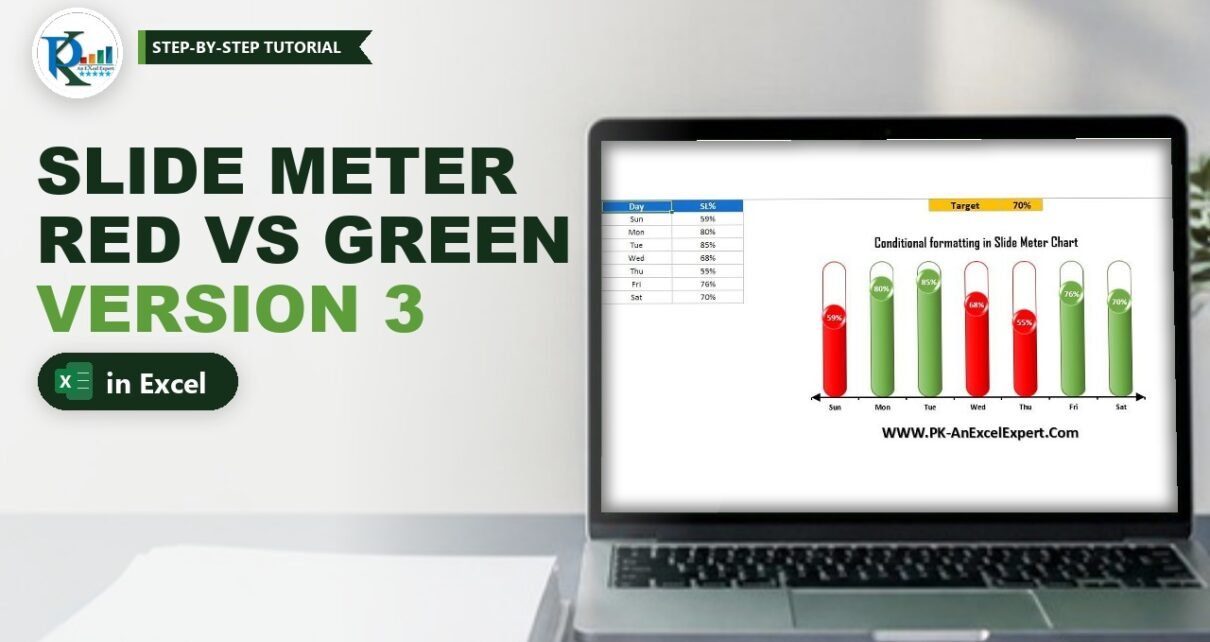
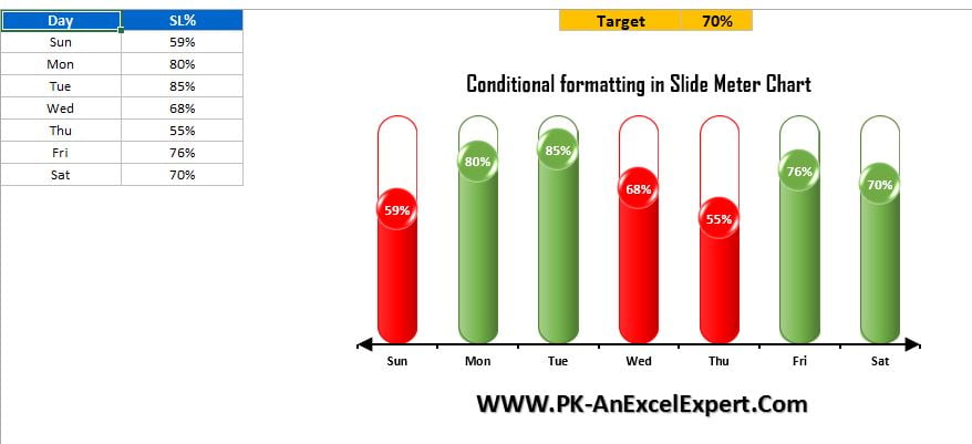
Conditional formatting in an Excel chart lets the colour of each bar react to a target: red when the KPI misses it, green when it hits it. This is Version 3 of PK’s slide meter chart. It keeps the semi-filled tracks from Version 2 and adds a target cell, four helper columns with IF and NA, and a red and a green set of shapes. Change the target or any value and the bars recolour themselves. No VBA.
Watch the Video Tutorial
In the video PK builds the target-based slide meter from a blank sheet: the four helper formulas, the six-series combo chart, the red and green shapes, Stack and Scale, and the coloured bubbles.
What You Will Build
- A target cell that controls the colour of every bar.
- Four helper columns that split each value into a green or a red series with IF and NA.
- Red and green semi-filled tracks, each with its own outlined 100% track.
- Red and green bubbles with white labels at the top of each fill.
- Automatic recolouring when you change the target or a value.
Part 1: Data, Target and Helper Columns
Step 1: Set up the table and the target
Start with the day-wise service level table in A1:B8 (Day and SL%) and turn off gridlines from the View tab. Type Target in J1 and the target value in K1. PK uses 75% in the video; the screenshot above uses 70%.
Add four helper headers: Green in C1, Red in D1, Max value for Green in E1 and Max value for Red in F1.
Step 2: Write the four formulas
C2  =IF(B2>=$K$1,B2,NA())
D2  =IF(B2<$K$1,B2,NA())
E2  =IF(B2>=$K$1,100%,NA())
F2  =IF(B2<$K$1,100%,NA())
Press F4 on the target reference so it becomes $K$1 and stays fixed when you copy down. Format C2:F2 as percentage and fill them down to row 8.
How the formulas work
- Green (C) returns the SL% only when it is greater than or equal to the target; otherwise
#N/A. - Red (D) returns the SL% only when it is below the target; otherwise
#N/A. - Max for Green (E) and Max for Red (F) return 100% on the same rows, so the empty track also takes the right colour.
NA()is the key: Excel charts skip#N/A, so each day draws only one colour. A zero would leave a stray marker at the bottom.
With a 75% target, Sunday at 70% gets 70% in Red and 100% in Max for Red, while Monday at 80% gets 80% in Green and 100% in Max for Green.
Part 2: Build the Combo Chart
Step 3: Insert the chart
Select A1:A8, hold Ctrl and select C1:F8, so the SL% column is skipped. Go to Insert › Column › 2-D Clustered Column.
Step 4: Fix the axis and gap width
Format the vertical axis with Minimum = 0 and Maximum = 1, then set the Gap Width to about 80%.
Step 5: Turn Green and Red into lines
Right-click a series, choose Change Series Chart Type and set Green and Red to Line with Markers. Keep both Max series as Clustered Column. These lines will carry the bubbles later.
Part 3: Red and Green Shapes
Step 6: Make the green pair
Draw a Rounded Rectangle, drag the yellow handle to round the ends, and give it a Gradient fill with the preset Medium Gradient – Accent 6 (green) and no outline. Copy it and set the copy to No Fill with a green theme outline. That is your filled and empty green track.
Step 7: Make the red pair
Copy both green shapes. On the filled one, change the gradient stops to a dark red, a red and a lighter custom red. Set the outline of the empty one to red.
Part 4: Conditional Formatting in the Excel Chart Series
Step 8: Add Green and Red again as columns
Copy the Green range (column C), click the chart and press Ctrl+V. Do the same with the Red range (column D). You now have Green and Red twice. Open Change Series Chart Type again: keep the first Green and Red as Line with Markers and set the second Green and Red to Clustered Column.
Step 9: Paste the shapes into the four column series
- Filled green pill into the Green column series.
- Filled red pill into the Red column series.
- Empty green pill into Max value for Green.
- Empty red pill into Max value for Red.
Step 10: Stack and Scale, then overlap
For each of the four column series open Format Data Series › Fill and choose Stack and Scale with, Units/Picture = 1. Because the axis runs from 0 to 1, a full pill equals 100%, so each fill is cut at its value instead of being squashed. Then set Series Overlap to 100% so every fill sits inside its track.
Delete the legend, the vertical axis and the gridlines. Select each line and set Shape Outline › No Outline, leaving only the markers.
Part 5: Coloured Bubbles and Finishing
Step 11: Red and green bubbles
Insert an Oval, fill it red, no outline, apply Shape Effects › Preset 5 and then Shadow › No Shadow, and size it 0.4 by 0.4. Copy it and make a green one. Paste the red oval on the Red markers and the green oval on the Green markers.
Step 12: Labels and axis
Add data labels to both marker series, set Label Position = Center, and make them white and bold. Make the day names black and bold, then give the axis line a black outline of about 2.25 pt with arrows from Shape Outline › Arrows. Add a title and test it: change the target in K1 and the bars switch colour instantly.
Common Errors and Fixes
A stray marker sits at 0%
A helper formula returns 0 or empty text instead of #N/A. Use NA() as the value-if-false.
All bars stay the same colour after changing the target
The target reference is not absolute. Re-enter it as $K$1 and fill the formulas down again.
The pills look squashed
One of the four column series is set to Stretch. Switch it to Stack and Scale with, Units/Picture 1, and check the axis maximum is 1.
The fills sit beside their tracks
Series Overlap is not 100%. Set it to 100% in Series Options.
Tips
- If your target changes every day, add a Target column and compare each row with its own target instead of
$K$1. - Want three bands (red, amber, green)? Add one more value column and one more Max column with their own IF rules and shapes.
- Put the target cell next to the chart and give it a fill colour, so users know where to change it.
- Microsoft’s page on the NA function explains why charts skip #N/A values.
The Slide Meter Chart Series
- Slide Meter Chart in Excel (Version 1): solid tracks with a sliding bubble.
- Semi-Filled Slide Meter Chart in Excel (Version 2): tracks that fill up to the value with Stack and Scale.
Want It Ready-Made?
To skip the build and use your own numbers right away, the Slide Meter Chart (Version-3) template is on NextGenTemplates.com, together with more Excel templates. To go deeper into dynamic charts and dashboards, take Excel Pivot Tables & Dashboards: Basic to Advanced on NextGenTemplates Academy.
Related Tutorials
- Conditional Formatting in Excel
- 5 KPI Cylinder Chart in Excel
- Thermometer Chart in Excel
- Dynamic Sales Score Meter Chart
Frequently Asked Questions
How do I apply conditional formatting to an Excel chart?
Charts do not have a conditional formatting menu, so you split the data into helper columns. One column keeps the value only when it meets the rule and the other keeps it only when it fails. Each column becomes its own series with its own colour, and Excel shows whichever one has a value.
Why use NA() instead of a blank or zero?
A zero would still draw a marker at the bottom of the chart, and an empty text result can be plotted as zero too. The #N/A error is skipped by Excel charts, so a day that does not belong to the green series simply shows nothing there.
Is a value equal to the target green or red?
Green. The green formulas use greater than or equal to the target, and the red formulas use less than the target. With a 70% target, 70% is green and 69% is red.
Can each day have a different target?
Yes. Add a Target column next to SL% and point the formulas to the target on the same row instead of the fixed cell K1. Each day is then compared with its own target.
What is the difference between Version 2 and Version 3?
Version 2 uses one colour and fills each track up to the value. Version 3 adds a target cell and two colour sets, so every bar switches between red and green automatically when the value or the target changes.
Does this chart need VBA?
No. The colour switch is done with IF and NA formulas in helper columns, and the design uses shapes pasted into chart series.
About the Author
PK is a Microsoft Excel expert and trainer and the founder of PK: An Excel Expert and NextGenTemplates.com. He has been teaching Excel, Power Query and Power BI since 2016 on his YouTube channel.
Conclusion
Conditional formatting in an Excel chart comes down to one idea: split each value into a pass series and a fail series with IF, hide the other with NA, and give each series its own colour. Combine that with the semi-filled tracks from Version 2 and you get a slide meter that turns red or green against your target automatically. Try changing the target and watch the whole chart respond.