Part of the free Module 10: Pivot Tables · Lesson 13 of 20 · Full Excel course
Updated on 5 September 2026 · Works in Excel 365, 2021, 2019 and 2016 unless noted.
A calculated field in a pivot table is a new value column built from a formula on other fields, such as Revenue divided by Sales. A calculated item is a new row or column entry built from other items of the same field, such as Q1 plus Q2. Both live under PivotTable Analyze > Fields, Items, & Sets.
Calculated field, calculated item, Show Values As or DAX measure
Four tools can add a number that is not in your source data, and picking the wrong one is the most common reason a pivot table shows a plausible but incorrect figure. Use this table before you open any dialog.
| Tool | What it creates | Calculated on | Use it for | Weakness |
|---|---|---|---|---|
| Calculated field | A new field in the Values area | The summed totals of each row of the report | Ratios and percentages: Revenue / Sales, Revenue * 5% | Cannot do row-by-row maths; ignores Average, Count and Min |
| Calculated item | A new item inside one row or column field | Other items of that same field | Combining or comparing categories: Q1+Q2, this year minus last year | Joins subtotals and grand totals, so it double counts |
| Show Values As | A different view of an existing field | The values already in the report | % of Grand Total, % of Parent Row, Difference From, Running Total | No custom arithmetic of your own |
| DAX measure (Data Model) | A measure in the Power Pivot model | Whatever grain you write, including row by row | Distinct count, weighted averages, SUMX, time intelligence | Needs Add this data to the Data Model when creating the pivot |
If your formula is a ratio of two totals, a calculated field is right. If it needs to run once per source row and then be summed, it belongs in the source data or in a DAX measure. See Value Field Settings and Show Values As and building a pivot table from multiple sheets with the Data Model.
How to add a calculated field
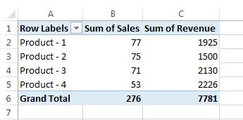
The starting pivot table shows product-wise Sum of Sales and Sum of Revenue but no revenue per sale.
- Click any cell inside the pivot table.
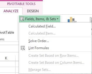
- Open the PivotTable Analyze tab (named Analyze in Excel 2016 and 2019, Options in Excel 2010), click Fields, Items, & Sets in the Calculations group and choose Calculated Field.
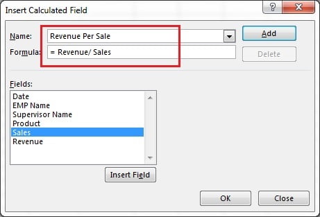
- In the Insert Calculated Field dialog type Revenue Per Sale in the Name box.
- Clear the Formula box and type
=, then double-click Revenue in the Fields list, type/and double-click Sales. The finished formula reads= Revenue / Sales. Double-clicking rather than typing avoids spelling errors and inserts the quotes that names with spaces need. - Click Add, then OK.
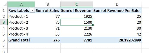
A column called Sum of Revenue Per Sale appears in the Values area, and the field itself joins the PivotTable Fields list so you can tick it on and off. Right-click the column and choose Value Field Settings > Number Format to show it as currency or with two decimals.
Formula rules inside the dialog
- Field names with spaces go in single quotes, for example
= 'Net Revenue' / 'Total Sales'. Double-clicking the field inserts the quotes for you. - No cell references and no ranges.
=B2*1.1or=SUM(A:A)are rejected. Only field names, item names, numbers and worksheet functions are allowed. - No references to other pivot tables or to grand totals. Use GETPIVOTDATA in a worksheet cell for that.
- Most worksheet functions work, including IF, IFERROR, ROUND, ABS and MAX, so
= IFERROR(Revenue / Sales, 0)is a safe version of the example above. Functions that need a range, such as SUMIF or COUNTIF, are not available. - The result is always summed. Excel labels it Sum of, and switching it to Average or Count in Value Field Settings changes the label without changing how the formula was worked out.
The trap: a calculated field multiplies the sums
This is the single biggest mistake with calculated fields. Excel does not calculate your formula on every source row and then total the answers. It totals each field first, then applies the formula once to those totals.
Suppose one product has three orders: 10 units at 5, 2 units at 50 and 4 units at 20. A calculated field = Price * Qty does not give 50 + 100 + 80 = 230. It gives Sum of Price (75) times Sum of Qty (16) = 1,200. The number is nonsense, yet nothing in the report warns you.
| Formula | What Excel computes | Correct? | Do this instead |
|---|---|---|---|
= Revenue / Sales |
Sum of Revenue / Sum of Sales | Yes, this is a weighted average and it is what you want | Nothing, keep the calculated field |
= Revenue * 0.05 |
Sum of Revenue * 0.05 | Yes, multiplying a total by a constant is safe | Nothing |
= Price * Qty |
Sum of Price * Sum of Qty | No, it is wildly overstated | Add a Line Total column to the source, or write a DAX measure with SUMX |
= AVERAGE(Margin) |
An average of the summed value, not of the rows | No | Put Margin in Values and set it to Average, or use a DAX measure |
Read the rule this way: totals in, formula once, answer out. An average of ratios computed at the total level, such as Revenue / Sales, is correct because that is genuinely what a weighted ratio means. Anything that must happen per source row belongs in the source data or in a Data Model measure, which is covered in Distinct Count with the Data Model.
How to add a calculated item
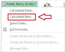
A calculated item adds a virtual member to a field, such as a Q1+Q2 row or a Product A minus Product B comparison line. The command stays greyed out until you click an actual item label.
- Click a Product label in the Row Labels area, not the header and not a value cell.
- Choose PivotTable Analyze > Fields, Items, & Sets > Calculated Item.
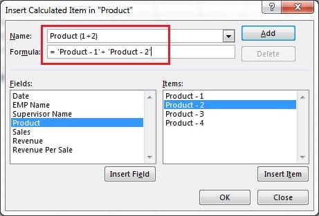
- Type Product (1+2) in the Name box.
- In the Formula box build
= 'Product - 1' + 'Product - 2'by double-clicking the entries in the Items list. Subtraction works the same way for a variance item, for example= 'Product - 1' - 'Product - 2'. - Click Add, then OK.
The new row appears among the products, with Sales and Revenue equal to the two originals combined. The item applies to every value field at once, which is convenient but also means you cannot switch it off for one measure only.
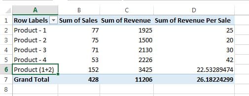
Two limits matter. First, the grand total now counts products 1 and 2 twice, once on their own rows and once inside the new item, so filter the originals out of the row field or turn the grand total off. Second, a field that carries a calculated item cannot be grouped, and a grouped field refuses new calculated items, which is why date grouping and calculated items never mix.
Solve order, List Formulas, modify and delete
When a cell sits where a calculated item and a calculated field cross, Excel has to decide which formula wins. Fields, Items, & Sets > Solve Order lists every item formula and lets you move one up or down; the last formula in the list is applied last and therefore controls the overlapping cell.
List Formulas writes a fresh worksheet documenting every calculated field and item with its formula and solve order. Print it or paste it into your documentation before handing the workbook over.
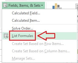
To change one, reopen the same dialog, pick the name from the Name drop-down, edit the formula and click Modify. To remove it, select the name and click Delete. Unticking a calculated field in the field list only hides it; the definition stays in the workbook until you delete it here.
Worked example
Take four rows of the practice file summarised by product:
| Product | Sum of Sales | Sum of Revenue | Revenue Per Sale |
|---|---|---|---|
| Product – 1 | 120 | 36,000 | 300 |
| Product – 2 | 80 | 28,000 | 350 |
| Product (1+2) | 200 | 64,000 | 320 |
The calculated field = Revenue / Sales gives 300 and 350 on the product rows. On the combined item it returns 64,000 / 200 = 320, not the simple average of 300 and 350, which would be 325. That difference is the weighting working correctly: product 1 sold more units, so it pulls the blended figure down. A grand total row would report 400 units and 128,000 revenue unless you hide the two original products.
Tips and common mistakes
- Never build a per-row product as a calculated field. Price times Qty, Hours times Rate and Units times Cost all need a helper column in the source data or a DAX measure.
- Hide the source items after adding a calculated item, or the grand total double counts them.
- Choose grouping or calculated items, not both. Ungroup the field first if Excel refuses the item.
- Wrap divisions in IFERROR so that products with zero sales show 0 instead of a divide-by-zero error across the report.
- Set the number format in Value Field Settings, not by formatting the cells, so it survives a refresh or a layout change.
- Run List Formulas before you inherit a workbook; a calculated field that someone added years ago is invisible until you look.
- Data Model pivots have neither command. If both options are greyed out, the pivot was created with Add this data to the Data Model and you need a measure instead.
Errors and how to fix them
| Message or symptom | Cause | Fix |
|---|---|---|
| The formula you typed contains an error | A cell reference, a misspelled field, or a name with spaces left unquoted | Rebuild the formula by double-clicking names in the Fields or Items list |
| Cannot add a calculated item when a field is grouped | The row or column field has grouped dates or numbers | Right-click the field, choose Ungroup, add the item, then decide which you need |
| Calculated Item is greyed out | No row or column item is selected, or the pivot uses the Data Model | Click an item label; for Data Model pivots write a DAX measure |
| #DIV/0! across a column | The denominator field totals zero for some rows | Change the formula to = IFERROR(Revenue / Sales, 0) |
| Grand total far too high | A calculated item is being added on top of its source items | Filter out the source items or switch the grand total off |
| Overlapping cell shows an unexpected number | A calculated field and a calculated item both apply there | Reorder the formulas in Solve Order |
Practice exercise
- Open the practice file, build a product-wise pivot with Sum of Sales and Sum of Revenue, then add the calculated field
= Revenue / Salesnamed Revenue Per Sale and format it to two decimals. - Add a second calculated field
= Revenue * 0.05named Commission and confirm the grand total commission equals five per cent of total revenue. - Put Supervisor in the Rows area and create a calculated item that subtracts one supervisor from another to show the gap between the two teams.
- Turn the grand total off, then on again, and note how the calculated item changes it.
- Run List Formulas and check that both fields and the item appear with the right solve order.
Key takeaways
- A calculated field adds a measure to the Values area; a calculated item adds a member to a row or column field.
- Calculated fields work on the summed totals, so ratios are correct and per-row products are not.
- Calculated items double count in subtotals and grand totals and cannot coexist with grouping.
- Formulas take field names, item names, constants and most worksheet functions, but never cell references.
- List Formulas documents everything; Solve Order settles cells where a field and an item overlap.
- For distinct counts, weighted per-row maths or time intelligence, use a Data Model DAX measure.
Related lessons
- Pivot Table course hub
- Value Field Settings: Sum, Average, Count and % share
- Distinct Count in a pivot table with the Data Model
- GETPIVOTDATA to pull pivot values into a report
- Pivot table from multiple sheets with relationships
- Excel formulas and functions module and SUMIFS for the worksheet alternative
- Microsoft: Calculate values in a PivotTable
Frequently asked questions
Why is my calculated field giving the wrong answer?
Because a calculated field totals each field first and then applies your formula once to those totals. Ratios such as Revenue divided by Sales are correct. Products such as Price times Quantity become Sum of Price times Sum of Quantity, which is far too high. Add that column to the source data or use a Data Model measure instead.
How do I delete a calculated field from a pivot table?
Open PivotTable Analyze, then Fields, Items, & Sets, then Calculated Field. Choose the field name from the Name drop-down and click Delete, then OK. Removing the tick in the field list only hides the column; the definition stays in the workbook until you delete it in this dialog.
Why is Calculated Item greyed out?
You must click an actual row or column item label first, not a header or a value cell. The command is also unavailable when the field is grouped, when the field is in the Values or Filters area, and when the pivot table is built on the Data Model. Ungroup the field, or write a DAX measure for Data Model pivots.
Can a calculated field use another calculated field?
Yes. Once a calculated field exists it appears in the Fields list of the dialog and can be used inside a later formula. Keep the chain short, because each layer still works on summed totals and errors compound quietly. List Formulas shows the whole chain and its solve order.
What is Solve Order used for?
Solve Order controls which formula wins in a cell where a calculated item and another calculated formula both apply. The formulas are applied in list order, so the last one determines the value shown. Open Fields, Items, & Sets, then Solve Order, and use Move Up or Move Down to change it.
Want the finished version? Ready-made Excel dashboards, trackers and VBA systems are available at NextGenTemplates.com.